Logistic map
The logistic map is a polynomial mapping (equivalently, recurrence relation) of degree 2, often cited as an archetypal example of how complex, chaotic behaviour can arise from very simple non-linear dynamical equations.[1] The map was popularized in a seminal 1976 paper by the biologist Robert May,[2] in part as a discrete-time demographic model analogous to the logistic equation first created by Pierre François Verhulst.[3] Mathematically, the logistic map is written

where is a number between zero and one that represents the ratio of existing population to the maximum possible population. The values of interest for the parameter are those in the interval . This nonlinear difference equation is intended to capture two effects:


![[0,4]](../I/m/74e35bf9a1852b3714b44393625cf4c127c946a7.svg)
- reproduction where the population will increase at a rate proportional to the current population when the population size is small.
- starvation (density-dependent mortality) where the growth rate will decrease at a rate proportional to the value obtained by taking the theoretical "carrying capacity" of the environment less the current population.
However, as a demographic model the logistic map has the pathological problem that some initial conditions and parameter values lead to negative population sizes. This problem does not appear in the older Ricker model, which also exhibits chaotic dynamics.
The case of the logistic map is a nonlinear transformation of both the bit-shift map and the case of the tent map.


Behavior dependent on
The image below shows the amplitude and frequency content of some logistic map iterates for parameter values ranging from 2 to 4.
By varying the parameter , the following behavior is observed:
- With between 0 and 1, the population will eventually die, independent of the initial population.
- With between 1 and 2, the population will quickly approach the value , independent of the initial population.
- With between 2 and 3, the population will also eventually approach the same value , but first will fluctuate around that value for some time. The rate of convergence is linear, except for , when it is dramatically slow, less than linear (see Bifurcation memory).
- With between 3 and , from almost all initial conditions the population will approach permanent oscillations between two values. These two values are dependent on .
- With between 3.44949 and 3.54409 (approximately), from almost all initial conditions the population will approach permanent oscillations among four values. The latter number is a root of a 12th degree polynomial (sequence A086181 in the OEIS).
- With increasing beyond 3.54409, from almost all initial conditions the population will approach oscillations among 8 values, then 16, 32, etc. The lengths of the parameter intervals that yield oscillations of a given length decrease rapidly; the ratio between the lengths of two successive such bifurcation intervals approaches the Feigenbaum constant . This behavior is an example of a period-doubling cascade.
- At (sequence A098587 in the OEIS) is the onset of chaos, at the end of the period-doubling cascade. From almost all initial conditions, we no longer see oscillations of finite period. Slight variations in the initial population yield dramatically different results over time, a prime characteristic of chaos.
- Most values of beyond 3.56995 exhibit chaotic behaviour, but there are still certain isolated ranges of that show non-chaotic behavior; these are sometimes called islands of stability. For instance, beginning at [4] (approximately 3.82843) there is a range of parameters that show oscillation among three values, and for slightly higher values of oscillation among 6 values, then 12 etc.
- The development of the chaotic behavior of the logistic sequence as the parameter varies from approximately 3.56995 to approximately 3.82843 is sometimes called the Pomeau–Manneville scenario, characterized by a periodic (laminar) phase interrupted by bursts of aperiodic behavior. Such a scenario has an application in semiconductor devices.[5] There are other ranges that yield oscillation among 5 values etc.; all oscillation periods occur for some values of . A period-doubling window with parameter is a range of -values consisting of a succession of sub-ranges. The th sub-range contains the values of for which there is a stable cycle (a cycle that attracts a set of initial points of unit measure) of period . This sequence of sub-ranges is called a cascade of harmonics.[6] In a sub-range with a stable cycle of period , there are unstable cycles of period for all . The value at the end of the infinite sequence of sub-ranges is called the point of accumulation of the cascade of harmonics. As rises there is a succession of new windows with different values. The first one is for ; all subsequent windows involving odd occur in decreasing order of starting with arbitrarily large .[6][7]
- Beyond , almost all initial values eventually leave the interval and diverge.


![[0,1]](../I/m/738f7d23bb2d9642bab520020873cccbef49768d.svg)
For any value of there is at most one stable cycle. If a stable cycle exists, it is globally stable, attracting almost all points.[8]:13 Some values of with a stable cycle of some period have infinitely many unstable cycles of various periods.
The bifurcation diagram at right summarizes this. The horizontal axis shows the possible values of the parameter while the vertical axis shows the set of values of visited asymptotically from almost all initial conditions by the iterates of the logistic equation with that value.

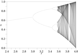
The bifurcation diagram is a self-similar: if you zoom in on the above-mentioned value and focus on one arm of the three, the situation nearby looks like a shrunk and slightly distorted version of the whole diagram. The same is true for all other non-chaotic points. This is an example of the deep and ubiquitous connection between chaos and fractals.

Chaos and the logistic map
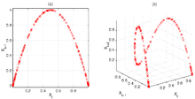


The relative simplicity of the logistic map makes it a widely used point of entry into a consideration of the concept of chaos.[1] A rough description of chaos is that chaotic systems exhibit a great sensitivity to initial conditions—a property of the logistic map for most values of between about 3.57 and 4 (as noted above).[9] A common source of such sensitivity to initial conditions is that the map represents a repeated folding and stretching of the space on which it is defined. In the case of the logistic map, the quadratic difference equation (1) describing it may be thought of as a stretching-and-folding operation on the interval .[10]

The following figure illustrates the stretching and folding over a sequence of iterates of the map. Figure (a), left, shows a two-dimensional Poincaré plot of the logistic map's state space for , and clearly shows the quadratic curve of the difference equation (1). However, we can embed the same sequence in a three-dimensional state space, in order to investigate the deeper structure of the map. Figure (b), right, demonstrates this, showing how initially nearby points begin to diverge, particularly in those regions of corresponding to the steeper sections of the plot.

This stretching-and-folding does not just produce a gradual divergence of the sequences of iterates, but an exponential divergence (see Lyapunov exponents), evidenced also by the complexity and unpredictability of the chaotic logistic map. In fact, exponential divergence of sequences of iterates explains the connection between chaos and unpredictability: a small error in the supposed initial state of the system will tend to correspond to a large error later in its evolution. Hence, predictions about future states become progressively (indeed, exponentially) worse when there are even very small errors in our knowledge of the initial state. This quality of unpredictability and apparent randomness led the logistic map equation to be used as a pseudo-random number generator in early computers.[10]
Since the map is confined to an interval on the real number line, its dimension is less than or equal to unity. Numerical estimates yield a correlation dimension of 0.500 ± 0.005 (Grassberger, 1983), a Hausdorff dimension of about 0.538 (Grassberger 1981), and an information dimension of 0.5170976... (Grassberger 1983) for (onset of chaos). Note: It can be shown that the correlation dimension is certainly between 0.4926 and 0.5024.

It is often possible, however, to make precise and accurate statements about the likelihood of a future state in a chaotic system. If a (possibly chaotic) dynamical system has an attractor, then there exists a probability measure that gives the long-run proportion of time spent by the system in the various regions of the attractor. In the case of the logistic map with parameter and an initial state in , the attractor is also the interval and the probability measure corresponds to the beta distribution with parameters and . Specifically,[11] the invariant measure is . Unpredictability is not randomness, but in some circumstances looks very much like it. Hence, and fortunately, even if we know very little about the initial state of the logistic map (or some other chaotic system), we can still say something about the distribution of states arbitrarily far into the future, and use this knowledge to inform decisions based on the state of the system.


Solution in some cases
The special case of can in fact be solved exactly, as can the case with [12] however the general case can only be predicted statistically.[13] The solution when is,[12][14]


where the initial condition parameter is given by . For rational , after a finite number of iterations maps into a periodic sequence. But almost all are irrational, and, for irrational , never repeats itself – it is non-periodic. This solution equation clearly demonstrates the two key features of chaos – stretching and folding: the factor shows the exponential growth of stretching, which results in sensitive dependence on initial conditions, while the squared sine function keeps folded within the range .


For an equivalent solution in terms of complex numbers instead of trigonometric functions is[15]

where is either of the complex numbers


with modulus equal to 1. Just as the squared sine function in the trigonometric solution leads to neither shrinkage nor expansion of the set of points visited, in the latter solution this effect is accomplished by the unit modulus of .
By contrast, the solution when is[15]

for . Since for any value of other than the unstable fixed point 0, the term goes to 0 as goes to infinity, so goes to the stable fixed point


Finding cycles of any length when
For the case, from almost all initial conditions the iterate sequence is chaotic. Nevertheless, there exist an infinite number of initial conditions that lead to cycles, and indeed there exist cycles of length for all integers . We can exploit the relationship of the logistic map to the dyadic transformation (also known as the bit-shift map) to find cycles of any length. If follows the logistic map and follows the dyadic transformation


then the two are related by
- .

The reason that the dyadic transformation is also called the bit-shift map is that when is written in binary notation, the map moves the binary point one place to the right (and if the bit to the left of the binary point has become a "1", this "1" is changed to a "0"). A cycle of length 3, for example, occurs if an iterate has a 3-bit repeating sequence in its binary expansion (which is not also a one-bit repeating sequence): 001, 010, 100, 110, 101, or 011. The iterate 001001001... maps into 010010010..., which maps into 100100100..., which in turn maps into the original 001001001...; so this is a 3-cycle of the bit shift map. And the other three binary-expansion repeating sequences give the 3-cycle 110110110... → 101101101... → 011011011... → 110110110.... Either of these 3-cycles can be converted to fraction form: for example, the first-given 3-cycle can be written as 1/7 → 2/7 → 4/7 → 1/7. Using the above translation from the bit-shift map to the logistic map gives the corresponding logistic cycle .611260467... → .950484434... → .188255099... → .611260467... . We could similarly translate the other bit-shift 3-cycle into its corresponding logistic cycle. Likewise, cycles of any length can be found in the bit-shift map and then translated into the corresponding logistic cycles.
However, since almost all numbers in are irrational, almost all initial conditions of the bit-shift map lead to the non-periodicity of chaos. This is one way to see that the logistic map is chaotic for almost all initial conditions.

The number of cycles of (minimal) length for the logistic map with (tent map with ) is a known integer sequence (sequence A001037 in the OEIS): 2, 1, 2, 3, 6, 9, 18, 30, 56, 99, 186, 335, 630, 1161 ... This tells us that the logistic map with has 2 fixed points, 1 cycle of length 2, 2 cycles of length 3 and so on. This sequence takes a particularly simple form for prime : . For example: is the number of cycles of length 13. Since this case of the logistic map is chaotic for almost all initial conditions, all of these finite-length cycles are unstable.


See also
- Logistic function, the continuous version
- Lyapunov stability#Definition for discrete-time systems
- Malthusian growth model
- Periodic points of complex quadratic mappings, of which the logistic map is a special case confined to the real line
- Radial basis function network, which illustrates the inverse problem for the logistic map.
- Schröder's equation (Not to be confused with Schrödinger's equation)
- Stiff equation
Notes
- 1 2 Boeing, G. (2016). "Visual Analysis of Nonlinear Dynamical Systems: Chaos, Fractals, Self-Similarity and the Limits of Prediction". Systems. 4 (4): 37. doi:10.3390/systems4040037. Retrieved 2016-12-02.
- ↑ May, Robert M. 1976. "Simple mathematical models with very complicated dynamics." Nature 261(5560):459-467.
- ↑ "Weisstein, Eric W. "Logistic Equation". MathWorld.
- ↑ Zhang, Cheng, "Period three begins", Mathematics Magazine 83, October 2010, 295-297.
- ↑ Carson Jeffries; Jose Perez (1982). "Observation of a Pomeau–Manneville intermittent route to chaos in a nonlinear oscillator". Physical Review A. 26 (4): 2117–2122. Bibcode:1982PhRvA..26.2117J. doi:10.1103/PhysRevA.26.2117.
- 1 2 R.M. May (1976). "Simple mathematical models with very complicated dynamics". Nature. 261 (5560): 459–67. Bibcode:1976Natur.261..459M. doi:10.1038/261459a0. PMID 934280.
- ↑ Baumol, William J; Benhabib, Jess (February 1989). "Chaos: Significance, Mechanism, and Economic Applications". Journal of Economic Perspectives. 3 (1): 77–105. doi:10.1257/jep.3.1.77.
- ↑ Collet, Pierre, and Jean-Pierre Eckmann, Iterated Maps on the Interval as Dynamical Systems, Birkhauser, 1980.
- ↑ May, Robert M. 1976. "Simple mathematical models with very complicated dynamics." Nature 261(5560):459-467.
- 1 2 Gleick, James (1987). Chaos: Making a New Science. Penguin Books.
- ↑ Jakobson, M.,"Absolutely continuous invariant measures for one-parameter families of one-dimensional maps," Communications in Mathematical Physics 81, 1981, 39-88.
- 1 2 Schröder, Ernst (1870). "Über iterierte Funktionen". Math. Ann. 3 (2): 296–322. doi:10.1007/BF01443992.
- ↑ Little, M.; Heesch, D. (2004). "Chaotic root-finding for a small class of polynomials" (PDF). Journal of Difference Equations and Applications. 10 (11): 949–953. doi:10.1080/10236190412331285351.
- ↑ Lorenz, Edward (1964), "The problem of deducing the climate from the governing equations," Tellus 16 (February): 1-11.
- 1 2 Schröder, Ernst (1870). "Ueber iterirte Functionen". Math. Ann. 3 (2): 296–322. doi:10.1007/BF01443992.
References
- P. Grassberger and I. Procaccia (1983). "Measuring the strangeness of strange attractors". Physica D. 9 (1–2): 189–208. Bibcode:1983PhyD....9..189G. doi:10.1016/0167-2789(83)90298-1.
- P. Grassberger (1981). "On the Hausdorff dimension of fractal attractors". Journal of Statistical Physics. 26 (1): 173–179. Bibcode:1981JSP....26..173G. doi:10.1007/BF01106792.
- Sprott, Julien Clinton (2003). Chaos and Time-Series Analysis. Oxford University Press. ISBN 0-19-850840-9.
- Strogatz, Steven (2000). Nonlinear Dynamics and Chaos. Perseus Publishing. ISBN 0-7382-0453-6.
- Tufillaro, Nicholas; Tyler Abbott; Jeremiah Reilly (1992). An experimental approach to nonlinear dynamics and chaos. Addison-Wesley New York. ISBN 0-201-55441-0.
External links
- Logistic Map Simulation. A Java applet simulating the Logistic Map by Yuval Baror.
- Logistic Map. Contains an interactive computer simulation of the logistic map.
- The Chaos Hypertextbook. An introductory primer on chaos and fractals.
- Interactive Logistic map with iteration and bifurcation diagrams in Java.
- Interactive Logistic map showing fixed points.
- Macintosh Quadratic Map Program
- The transition to Chaos and the Feigenbaum constant- JAVA applet
- The Logistic Map and Chaos by Elmer G. Wiens
- Complexity & Chaos (audiobook) by Roger White. Chapter 5 covers the Logistic Equation.
- "History of iterated maps," in A New Kind of Science by Stephen Wolfram. Champaign, IL: Wolfram Media, p. 918, 2002.
- Discrete Logistic Equation by Marek Bodnar after work by Phil Ramsden, Wolfram Demonstrations Project.
- Multiplicative coupling of 2 logistic maps by C. Pellicer-Lostao and R. Lopez-Ruiz after work by Ed Pegg Jr, Wolfram Demonstrations Project.
- Using SAGE to investigate the discrete logistic equation