Low-discrepancy sequence

In mathematics, a low-discrepancy sequence is a sequence with the property that for all values of N, its subsequence x₁, ..., x_N has a low discrepancy.

Roughly speaking, the discrepancy of a sequence is low if the proportion of points in the sequence falling into an arbitrary set B is close to proportional to the measure of B, as would happen on average (but not for particular samples) in the case of an equidistributed sequence. Specific definitions of discrepancy differ regarding the choice of B (hyperspheres, hypercubes, etc.) and how the discrepancy for every B is computed (usually normalized) and combined (usually by taking the worst value).

Low-discrepancy sequences are also called quasi-random or sub-random sequences, due to their common use as a replacement of uniformly distributed random numbers. The "quasi" modifier is used to denote more clearly that the values of a low-discrepancy sequence are neither random nor pseudorandom, but such sequences share some properties of random variables and in certain applications such as the quasi-Monte Carlo method their lower discrepancy is an important advantage.

Applications

Error in estimated kurtosis as a function of number of datapoints. 'Additive subrandom' gives the maximum error when c = (√5 − 1)/2. 'Random' gives the average error over six runs of random numbers, where the average is taken to reduce the magnitude of the wild fluctuations

Subrandom numbers have an advantage over pure random numbers in that they cover the domain of interest quickly and evenly. They have an advantage over purely deterministic methods in that deterministic methods only give high accuracy when the number of datapoints is pre-set whereas in using subrandom sequences the accuracy typically improves continually as more datapoints are added, with full reuse of the existing points. On the other hand, subrandom sets can have a significant lower discrepancy for a given number of points than subrandom sequences.

Two useful applications are in finding the characteristic function of a probability density function, and in finding the derivative function of a deterministic function with a small amount of noise. Subrandom numbers allow higher-order moments to be calculated to high accuracy very quickly.

Applications that don't involve sorting would be in finding the mean, standard deviation, skewness and kurtosis of a statistical distribution, and in finding the integral and global maxima and minima of difficult deterministic functions. Subrandom numbers can also be used for providing starting points for deterministic algorithms that only work locally, such as Newton–Raphson iteration.

Subrandom numbers can also be combined with search algorithms. A binary tree Quicksort-style algorithm ought to work exceptionally well because subrandom numbers flatten the tree far better than random numbers, and the flatter the tree the faster the sorting. With a search algorithm, subrandom numbers can be used to find the mode, median, confidence intervals and cumulative distribution of a statistical distribution, and all local minima and all solutions of deterministic functions.

Low-discrepancy sequences in numerical integration

At least three methods of numerical integration can be phrased as follows. Given a set {x₁, ..., x_N} in the interval [0,1], approximate the integral of a function f as the average of the function evaluated at those points:

$\int _{0}^{1}f(u)\,du\approx {\frac {1}{N}}\,\sum _{{i=1}}^{N}f(x_{i}).$

If the points are chosen as x_i = i/N, this is the rectangle rule. If the points are chosen to be randomly (or pseudorandomly) distributed, this is the Monte Carlo method. If the points are chosen as elements of a low-discrepancy sequence, this is the quasi-Monte Carlo method. A remarkable result, the Koksma–Hlawka inequality (stated below), shows that the error of such a method can be bounded by the product of two terms, one of which depends only on f, and the other one is the discrepancy of the set {x₁, ..., x_N}.

It is convenient to construct the set {x₁, ..., x_N} in such a way that if a set with N+1 elements is constructed, the previous N elements need not be recomputed. The rectangle rule uses points set which have low discrepancy, but in general the elements must be recomputed if N is increased. Elements need not be recomputed in the random Monte Carlo method if N is increased, but the point sets do not have minimal discrepancy. By using low-discrepancy sequences we aim for low discrepancy and no need for recomputations, but actually LDS can only be incrementally good on discrepancy if we allow no recomputation.

Definition of discrepancy

The discrepancy of a set P = {x₁, ..., x_N} is defined, using Niederreiter's notation, as

$D_{N}(P)=\sup _{{B\in J}}\left|{\frac {A(B;P)}{N}}-\lambda _{s}(B)\right|$

where λ_s is the s-dimensional Lebesgue measure, A(B;P) is the number of points in P that fall into B, and J is the set of s-dimensional intervals or boxes of the form

$\prod _{{i=1}}^{s}[a_{i},b_{i})=\{{\mathbf {x}}\in {\mathbf {R}}^{s}:a_{i}\leq x_{i}<b_{i}\}\,$

where $0\leq a_{i}<b_{i}\leq 1$.

The star-discrepancy D^*_N(P) is defined similarly, except that the supremum is taken over the set J^* of rectangular boxes of the form

$\prod _{{i=1}}^{s}[0,u_{i})$

where u_i is in the half-open interval [0, 1).

The two are related by

$D_{N}^{*}\leq D_{N}\leq 2^{s}D_{N}^{*}.\,$

The Koksma–Hlawka inequality

Let Ī^s be the s-dimensional unit cube, Ī^s = [0, 1] × ... × [0, 1]. Let f have bounded variation V(f) on Ī^s in the sense of Hardy and Krause. Then for any x₁, ..., x_N in I^s = [0, 1) × ... × [0, 1),

$\left|{\frac {1}{N}}\sum _{{i=1}}^{N}f(x_{i})-\int _{{{\bar I}^{s}}}f(u)\,du\right|\leq V(f)\,D_{N}^{*}(x_{1},\ldots ,x_{N}).$

The Koksma–Hlawka inequality is sharp in the following sense: For any point set {x₁,...,x_N} in I^s and any $\varepsilon >0$, there is a function f with bounded variation and V(f) = 1 such that

${\displaystyle \left|{\frac {1}{N}}\sum _{i=1}^{N}f(x_{i})-\int _{{\bar {I}}^{s}}f(u)\,du\right|>D_{N}^{*}(x_{1},\ldots ,x_{N})-\varepsilon .}$

Therefore, the quality of a numerical integration rule depends only on the discrepancy D^*_N(x₁,...,x_N).

The formula of Hlawka–Zaremba

Let $D=\{1,2,\ldots ,d\}$. For $\emptyset \neq u\subseteq D$ we write

$dx_{u}:=\prod _{{j\in u}}dx_{j}$

and denote by $(x_{u},1)$ the point obtained from x by replacing the coordinates not in u by $1$. Then

${\displaystyle {\frac {1}{N}}\sum _{i=1}^{N}f(x_{i})-\int _{{\bar {I}}^{s}}f(u)\,du=\sum _{\emptyset \neq u\subseteq D}(-1)^{|u|}\int _{[0,1]^{|u|}}\operatorname {disc} (x_{u},1){\frac {\partial ^{|u|}}{\partial x_{u}}}f(x_{u},1)\,dx_{u},}$

where ${\displaystyle \operatorname {disc} (z)={\frac {1}{N}}\sum _{i=1}^{N}\prod _{j=1}^{d}1_{[0,z_{j})}(x_{i,j})-\prod _{j=1}^{d}z_{i}}$ is the discrepancy function.

The $L^{2}$ version of the Koksma–Hlawka inequality

Applying the Cauchy–Schwarz inequality for integrals and sums to the Hlawka–Zaremba identity, we obtain an $L^{2}$ version of the Koksma–Hlawka inequality:

${\displaystyle \left|{\frac {1}{N}}\sum _{i=1}^{N}f(x_{i})-\int _{{\bar {I}}^{s}}f(u)\,du\right|\leq \|f\|_{d}\operatorname {disc} _{d}(\{t_{i}\}),}$

where

${\displaystyle \operatorname {disc} _{d}(\{t_{i}\})=\left(\sum _{\emptyset \neq u\subseteq D}\int _{[0,1]^{|u|}}\operatorname {disc} (x_{u},1)^{2}\,dx_{u}\right)^{1/2}}$

and

${\displaystyle \|f\|_{d}=\left(\sum _{u\subseteq D}\int _{[0,1]^{|u|}}\left|{\frac {\partial ^{|u|}}{\partial x_{u}}}f(x_{u},1)\right|^{2}dx_{u}\right)^{1/2}.}$

The Erdős–Turán–Koksma inequality

It is computationally hard to find the exact value of the discrepancy of large point sets. The Erdős–Turán–Koksma inequality provides an upper bound.

Let x₁,...,x_N be points in I^s and H be an arbitrary positive integer. Then

$D_{{N}}^{{*}}(x_{1},\ldots ,x_{N})\leq \left({\frac {3}{2}}\right)^{s}\left({\frac {2}{H+1}}+\sum _{{0<\|h\|_{{\infty }}\leq H}}{\frac {1}{r(h)}}\left|{\frac {1}{N}}\sum _{{n=1}}^{{N}}e^{{2\pi i\langle h,x_{n}\rangle }}\right|\right)$

where

$r(h)=\prod _{{i=1}}^{s}\max\{1,|h_{i}|\}\quad {\mbox{for}}\quad h=(h_{1},\ldots ,h_{s})\in \mathbb{Z } ^{s}.$

The main conjectures

Conjecture 1. There is a constant c_s depending only on the dimension s, such that

$D_{{N}}^{{*}}(x_{1},\ldots ,x_{N})\geq c_{s}{\frac {(\ln N)^{{s-1}}}{N}}$

for any finite point set {x₁,...,x_N}.

Conjecture 2. There is a constant c^'_s depending only on s, such that

$D_{{N}}^{{*}}(x_{1},\ldots ,x_{N})\geq c'_{s}{\frac {(\ln N)^{{s}}}{N}}$

for at least one N for any infinite sequence x₁,x₂,x₃,....

These conjectures are equivalent. They have been proved for s ≤ 2 by W. M. Schmidt. In higher dimensions, the corresponding problem is still open. The best-known lower bounds are due to K. F. Roth.

Lower bounds

Let s = 1. Then

$D_{N}^{*}(x_{1},\ldots ,x_{N})\geq {\frac {1}{2N}}$

for any finite point set {x₁, ..., x_N}.

Let s = 2. W. M. Schmidt proved that for any finite point set {x₁, ..., x_N},

$D_{N}^{*}(x_{1},\ldots ,x_{N})\geq C{\frac {\log N}{N}}$

where

$C=\max _{{a\geq 3}}{\frac {1}{16}}{\frac {a-2}{a\log a}}=0.023335\dots$

For arbitrary dimensions s > 1, K.F. Roth proved that

$D_{N}^{*}(x_{1},\ldots ,x_{N})\geq {\frac {1}{2^{{4s}}}}{\frac {1}{((s-1)\log 2)^{{\frac {s-1}{2}}}}}{\frac {\log ^{{{\frac {s-1}{2}}}}N}{N}}$

for any finite point set {x₁, ..., x_N}. This bound is the best known for s > 3.

Construction of low-discrepancy sequences

Because any distribution of random numbers can be mapped onto a uniform distribution, and subrandom numbers are mapped in the same way, this article only concerns generation of subrandom numbers on a multidimensional uniform distribution.

There are constructions of sequences known such that

${\displaystyle D_{N}^{*}(x_{1},\ldots ,x_{N})\leq C{\frac {(\ln N)^{s}}{N}}.}$

where C is a certain constant, depending on the sequence. After Conjecture 2, these sequences are believed to have the best possible order of convergence. Examples below are the van der Corput sequence, the Halton sequences, and the Sobol sequences.

Random numbers

Sequences of subrandom numbers can be generated from random numbers by imposing a negative correlation on those random numbers. One way to do this is to start with a set of random numbers $r_{i}$ on $[0,0.5)$ and construct subrandom numbers $s_{i}$ which are uniform on $[0,1)$ using:

$s_{i}=r_{i}$ for $i$ odd and $s_{i}=0.5+r_{i}$ for $i$ even.

A second way to do it with the starting random numbers is to construct a random walk with offset 0.5 as in:

$s_{i}=s_{{i-1}}+0.5+r_{i}{\pmod 1}.\,$

That is, take the previous subrandom number, add 0.5 and the random number, and take the result modulo 1.

For more than one dimension, Latin squares of the appropriate dimension can be used to provide offsets to ensure that the whole domain is covered evenly.

Coverage of the unit square. Left for additive subrandom numbers with c = 0.5545497..., 0.308517... Right for random numbers. From top to bottom. 10, 100, 1000, 10000 points.

Additive recurrence

For any irrational $\alpha$, the sequence

$s_{n}=\{s_{0}+n\alpha \}$

has discrepancy tending to 0. (Note the sequence can be defined recursively by $s_{{n+1}}=(s_{n}+\alpha ){\bmod \,}1$.) A good value of $\alpha$ gives lower discrepancy than a sequence of independent uniform random numbers.

The discrepancy can be bounded by the approximation exponent of $\alpha$. If the approximation exponent is $\mu$, then for any $\varepsilon >0$, the following bound holds:^[1]

${\displaystyle D_{N}((s_{n}))=O_{\varepsilon }(N^{-1/(\mu -1)+\varepsilon }).}$

By the Thue–Siegel–Roth theorem, the approximation exponent of any irrational algebraic number is 2, giving a bound of ${\displaystyle N^{-1+\varepsilon }}$ above.

The value of $c$ with lowest discrepancy is ^[2]

$c={\frac {{\sqrt {5}}-1}{2}}\approx 0.618034.$

Another value that is nearly as good is:

$c={\sqrt {2}}-1\approx 0.414214.\,$

In more than one dimension, separate subrandom numbers are needed for each dimension. In higher dimensions, one set of values that can be used is the square roots of primes from two up, all taken modulo 1:

$c={\sqrt {2}},{\sqrt {3}},{\sqrt {5}},{\sqrt {7}},{\sqrt {11}},\ldots \,$

The recurrence relation above is similar to the recurrence relation used by a Linear congruential generator, a poor-quality pseudorandom number generator:^[3]

$r_{i}={\bmod (}ar_{{i-1}}+c,m)$

For the low discrepancy additive recurrence above, a and m are chosen to be 1. Note, however, that this will not generate independent random numbers, so should not be used for purposes requiring independence. The list of pseudorandom number generators lists methods for generating independent pseudorandom numbers.

van der Corput sequence

Let

$n=\sum _{{k=0}}^{{L-1}}d_{k}(n)b^{k}$

be the b-ary representation of the positive integer n ≥ 1, i.e. 0 ≤ d_k(n) < b. Set

$g_{b}(n)=\sum _{{k=0}}^{{L-1}}d_{k}(n)b^{{-k-1}}.$

Then there is a constant C depending only on b such that (g_b(n))_{n ≥ 1}satisfies

$D_{N}^{*}(g_{b}(1),\dots ,g_{b}(N))\leq C{\frac {\log N}{N}},$

where D^*_N is the star discrepancy.

Halton sequence

First 256 points of the (2,3) Halton sequence

The Halton sequence is a natural generalization of the van der Corput sequence to higher dimensions. Let s be an arbitrary dimension and b₁, ..., b_s be arbitrary coprime integers greater than 1. Define

$x(n)=(g_{{b_{1}}}(n),\dots ,g_{{b_{s}}}(n)).$

Then there is a constant C depending only on b₁, ..., b_s, such that sequence {x(n)}_n≥1 is a s-dimensional sequence with

$D_{N}^{*}(x(1),\dots ,x(N))\leq C'{\frac {(\log N)^{s}}{N}}.$

Hammersley set

2D Hammersley set of size 256

Let b₁,...,b_s-1 be coprime positive integers greater than 1. For given s and N, the s-dimensional Hammersley set of size N is defined by^[4]

$x(n)=(g_{{b_{1}}}(n),\dots ,g_{{b_{{s-1}}}}(n),{\frac {n}{N}})$

for n = 1, ..., N. Then

$D_{N}^{*}(x(1),\dots ,x(N))\leq C{\frac {(\log N)^{{s-1}}}{N}}$

where C is a constant depending only on b₁, ..., b_s−1.

Sobol sequence

The Antonov–Saleev variant of the Sobol sequence generates numbers between zero and one directly as binary fractions of length $w$, from a set of $w$ special binary fractions, $V_{i},i=1,2,\dots ,w$ called direction numbers. The bits of the Gray code of $i$, $G(i)$, are used to select direction numbers. To get the Sobol sequence value $s_{i}$ take the exclusive or of the binary value of the Gray code of$i$ with the appropriate direction number. The number of dimensions required affects the choice of $V_{i}$.

Poisson disk sampling

Poisson disk sampling is popular in video games to rapidly placing objects in a way that appears random-looking but guarantees that every two points are separated by at least the specified minimum distance.^[5]

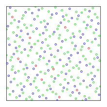
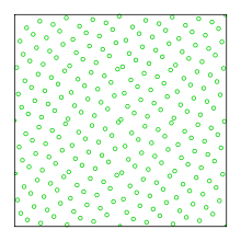
Graphical examples

The points plotted below are the first 100, 1000, and 10000 elements in a sequence of the Sobol' type. For comparison, 10000 elements of a sequence of pseudorandom points are also shown. The low-discrepancy sequence was generated by TOMS algorithm 659.^[6] An implementation of the algorithm in Fortran is available from Netlib.

See also

• Discrepancy theory
• Quasi-Monte Carlo method
• Markov chain Monte Carlo
• Sparse grid

References

1. Kuipers and Niederreiter, 2005, p. 123
2. http://mollwollfumble.blogspot.com/, Subrandom numbers
3. Donald E. Knuth The Art of Computer Programming Vol. 2, Ch. 3
4. Hammersley, J. M.; Handscomb, D. C. (1964). Monte Carlo Methods. doi:10.1007/978-94-009-5819-7.
5. Herman Tulleken. "Poisson Disk Sampling". Dev.Mag Issue 21, March 2008.
6. P. Bratley and B.L. Fox in ACM Transactions on Mathematical Software, vol. 14, no. 1, pp 88—100

• Josef Dick and Friedrich Pillichshammer, Digital Nets and Sequences. Discrepancy Theory and Quasi-Monte Carlo Integration, Cambridge University Press, Cambridge, 2010, ISBN 978-0-521-19159-3
• Kuipers, L.; Niederreiter, H. (2005), Uniform distribution of sequences, Dover Publications, ISBN 0-486-45019-8
• Harald Niederreiter. Random Number Generation and Quasi-Monte Carlo Methods. Society for Industrial and Applied Mathematics, 1992. ISBN 0-89871-295-5
• Michael Drmota and Robert F. Tichy, Sequences, discrepancies and applications, Lecture Notes in Math., 1651, Springer, Berlin, 1997, ISBN 3-540-62606-9
• William H. Press, Brian P. Flannery, Saul A. Teukolsky, William T. Vetterling. Numerical Recipes in C. Cambridge, UK: Cambridge University Press, second edition 1992. ISBN 0-521-43108-5 (see Section 7.7 for a less technical discussion of low-discrepancy sequences)

External links

• Collected Algorithms of the ACM (See algorithms 647, 659, and 738.)
• GNU Scientific Library Quasi-Random Sequences
• Quasi-random sampling subject to constraints at FinancialMathematics.Com
• C++ generator of Sobol sequence