Monopoly price
A monopoly price is set by a monopoly.[1][2] A monopoly occurs when a firm is the only firm in an industry producing the product, such that the monopoly faces no competition.[1][2] A monopoly has absolute market power, and thereby can set a monopoly price that will be above the firm's marginal (economic) cost, which is the change in total (economic) cost due to one additional unit produced.[1]
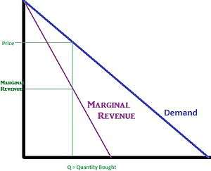
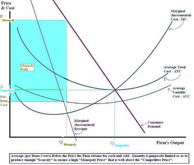
The monopoly will ensure a monopoly price will exist when it establishes the quantity of the product it will sell.[1] As the sole supplier of the product within the market, its sales establish the entire industry's supply within the market, and therefore the monopoly's production and sales decisions can establish a single monopoly price for the industry without any influence from competing firms.[1][2][3] The monopoly will always consider the demand for its product as it considers what price is appropriate; such that it will choose a production supply and price combination that will ensure a maximum economic profit.[1][2] It does this by ensuring the marginal cost (determined by the firm's technical limitations that form its cost structure) is the same as the marginal revenue (as determined by the impact a change in the price of the product will impact the quantity demanded) at the quantity it decides to sell.[1][2] The marginal revenue is solely determined by the demand for the product within the industry, and is the change in revenue that will occur by lowering the price just enough to ensure a single additional unit will be sold.[1][2] The marginal revenue is positive, but it is lower than the price associated with it because lowering the price will:
- (a) increase the demand for its product, thereby increasing the firm's Sales Revenue,[1] and
- (b) Lower the price paid by those who were willing to buy the product at the higher price, thereby ensuring a lower Sales Revenue on the Product Sales to those who were willing to pay the higher price.[1]

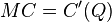
"Marginal Cost" solely relates to the firm's technical "Cost Structure" within production, and indicates the rise in Total (Economic) Cost that must occur for an additional unit to be supplied to the market by the firm.[1] "Marginal Cost" is higher than "Average Cost" because of the existence of "Diminishing Marginal Product" in the "Short Run".[1]
- Marginal Cost =
 [2]
[2] - where
 [2][4]
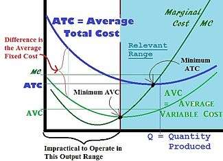 Diminishing Marginal Product ensures the Rise in Cost from producing an additional Item (Marginal Cost) is always greater than the Average Variable (Controllable) Cost at that level of production. Since some costs cannot be controlled in the "Short Run", the Variable (Controllable) Costs will always be lower than the Total Costs in the "Short Run".
- Marginal Cost =
Samuelson indicates this point on the Consumer Demand curve is where Price is equal to one over one plus the reciprocal of the price elasticity of demand.[5] This rule does not apply to competitive firms since such firms are price takers, and don't have the market power to control either prices or Industry-Wide Sales.[1]
Although the term "markup" is sometimes used in economics to refer to difference between a Monopoly Price and the Monopoly's Marginal Cost (MC),[6] the term markup is frequently used in American Accounting and Finance to define the difference between the Price of the Product and its per unit Accounting Cost. Accepted Neo-Classical Micro-Economic Theory indicates the American Accounting and Finance definition of markup, as it exists in most Competitive Markets, solely ensures an "Accounting Profit" that will be just enough to solely compensate the Equity owners of a "Competitive Firm" within a "Competitive Market" for the "Economic Cost" ("Opportunity Cost") they must bear when they decide to hold on to the Firm's Equity.[3] The "Economic Cost" of holding onto Equity at its Present Value is the "Opportunity Cost" the Investor must bare when he gives up the Interest Earnings on Debt of similar Present Value (He holds onto Equity instead of the Debt).[3] Economists would indicate a Markup rule on Economic Cost used by a Monopoly to set a "Monopoly Price" that will maximize its Profit, is excessive markup that leads to inefficiencies within an economic system.[1][2][7][8]
Mathematical Derivation - How a Monopoly Sets the Monopoly Price
Mathematically, we derive the general rule a Monopoly uses to maximize Monopoly profit through simple Calculus. We first depict the basic equation for "Economic Profit", in which the Total Economic Cost varies directly with the quantity produced:
- where
- Q = quantity sold,
- P(Q) = inverse demand function, and thereby the Price at which Q can be sold given the existing Demand
- C(Q) = Total (Economic) Cost of producing Q.
 = Economic Profit
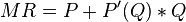
This is done by setting the derivative of with respect to Q equal to 0, Profit of a firm is given by total revenue (price times quantity sold) minus total cost:
- where
- Q = quantity sold,
- P'(Q) = the partial derivative of the inverse demand function, and thereby the Price at which Q can be sold given the existing Demand
- C'(Q) = Marginal Cost, or the partial derivative of the Total (Economic) Cost of producing Q.
This yields:

or "Marginal Revenue" = "Marginal Cost". This is usually called the "First Order Conditions" for a Profit Maximum.[2]
According to Samuelson,
By definition  is the reciprocal of the price elasticity of demand (or
  ). Hence
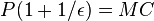
This gives the markup rule:
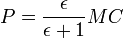
or, letting  be the reciprocal of the price elasticity of demand,
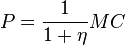
Thus the monopolistic firm chooses the quantity at which the demand price satisfies this rule. Since for a price setting firm  this means that a firm with market power will charge a price above marginal cost and thus earn a monopoly rent. On the other hand, a competitive firm by definition faces a perfectly elastic demand, hence it believes
  which means that it sets price equal to marginal cost.
The rule also implies that, absent menu costs, a monopolistic firm will never choose a point on the inelastic portion of its demand curve. Furthermore, for an equilibrium to exist in a monopoly or in an oligopoly market, the price elasticity of demand must be less than negative one ( )(Mas-Colell) simply because the price elasticity of demand must be less than negative one for Marginal Revenue (MR) to be positive.[4] The Mathematical Profit Maximization Conditions ("First Order Conditions") ensure the price elasticity of demand must be less than negative one;[2][7] since no "Rational Firm" that attempts to maximize its profit would incur additional Cost (a positive Marginal Cost) in order to Reduce Revenue (when MR < 0).[1]
References
- 1 2 3 4 5 6 7 8 9 10 11 12 13 14 15 Roger LeRoy Miller, Intermediate Microeconomics Theory Issues Applications, Third Edition, New York: McGraw-Hill, Inc, 1982.
- 1 2 3 4 5 6 7 8 9 10 11 12 13 Tirole, Jean, "The Theory of Industrial Organization", Cambridge, Massachusetts: The MIT Press, 1988.
- 1 2 3 John Black, "Oxford Dictionary of Economics", New York: Oxford University Press, 2003.
- 1 2 Henderson, James M., and Richard E. Quandt, "Micro Economic Theory, A Mathematical Approach. 3rd Edition", New York: McGraw-Hill Book Company, 1980. Glenview, Illinois: Scott, Foresmand and Company, 1988.
- Usually, in many Text Books, Economic Cost, here presented by C(Q), is divided into 2 Categories; Labor Costs and Capital Costs:
- C(Q) = L * w + K * R
- where
- Usually, in many Text Books, Economic Cost, here presented by C(Q), is divided into 2 Categories; Labor Costs and Capital Costs:
- ↑ Samuelson; Marks (2003). p.104
- ↑ Nicholson, Walter and Christopher Snyder, Microeconomic Theory: Basic Principles and Extensions, Mason, OH: Thomson/South-Western, 2008.
- 1 2 Henderson, James M., and Richard E. Quandt, "Micro Economic Theory, A Mathematical Approach. 3rd Edition", New York: McGraw-Hill Book Company, 1980. Glenview, Illinois: Scott, Foresmand and Company, 1988.
- ↑ Bradley R. chiller, "Essentials of Economics", New York: McGraw-Hill, Inc., 1991.