Radial trajectory
In astrodynamics and celestial mechanics a radial trajectory is a Kepler orbit with zero angular momentum. Two objects in a radial trajectory move directly towards or away from each other in a straight line.
Classification
There are three types of radial trajectories (orbits).[1]
- Radial elliptic trajectory: an orbit corresponding to the part of a degenerate ellipse from the moment the bodies touch each other and move away from each other until they touch each other again. The relative speed of the two objects is less than the escape velocity. This is an elliptic orbit with semi-minor axis = 0 and eccentricity = 1. Although the eccentricity is 1 this is not a parabolic orbit. If the coefficient of restitution of the two bodies is 1 (perfectly elastic) this orbit is periodic. If the coefficient of restitution is less than 1 (inelastic) this orbit is non-periodic.
- Radial parabolic trajectory, a non-periodic orbit where the relative speed of the two objects is always equal to the escape velocity. There are two cases: the bodies move away from each other or towards each other.
- Radial hyperbolic trajectory: a non-periodic orbit where the relative speed of the two objects always exceeds the escape velocity. There are two cases: the bodies move away from each other or towards each other. This is a hyperbolic orbit with semi-minor axis = 0 and eccentricity = 1. Although the eccentricity is 1 this is not a parabolic orbit.
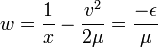
Unlike standard orbits which are classified by their orbital eccentricity, radial orbits are classified by their specific orbital energy, the constant sum of the total kinetic and potential energy, divided by the reduced mass:

where x is the distance between the centers of the masses, v is the relative velocity, and  is the standard gravitational parameter.
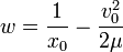
Another constant is given by:
- For elliptic trajectories, w is positive. It is the inverse of the apoapsis distance (maximum distance).
- For parabolic trajectories, w is zero.
- For hyperbolic trajectories, w is negative, It is
 where
where  is the velocity at infinite distance.
Time as a function of distance
Given the separation and velocity at any time, and the total mass, it is possible to determine the position at any other time.
The first step is to determine the constant w. Use the sign of w to determine the orbit type.
where  and
and  are the separation and relative velocity at any time.
Parabolic trajectory
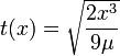
where t is the time from or until the time at which the two masses, if they were point masses, would coincide, and x is the separation.
This equation applies only to radial parabolic trajectories, for general parabolic trajectories see Barker's equation.
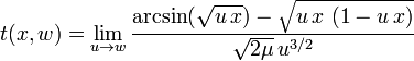
Elliptic trajectory
where t is the time from or until the time at which the two masses, if they were point masses, would coincide, and x is the separation.
This is the radial Kepler equation.[2]
See also equations for a falling body.
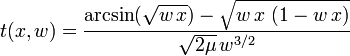
Hyperbolic trajectory
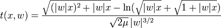
where t is the time from or until the time at which the two masses, if they were point masses, would coincide, and x is the separation.
Universal form (any trajectory)
The radial Kepler equation can be made "universal" (applicable to all trajectories):
or by expanding in a power series:

The radial Kepler problem (distance as function of time)
The problem of finding the separation of two bodies at a given time, given their separation and velocity at another time, is known as the Kepler problem. This section solves the Kepler problem for radial orbits.
The first step is to determine the constant w. Use the sign of w to determine the orbit type.
Where and are the separation and velocity at any time.
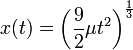
Parabolic trajectory
See also position as function of time in a straight escape orbit.
Universal form (any trajectory)
Two intermediate quantities are used: w, and the separation at time t the bodies would have if they were on a parabolic trajectory, p.
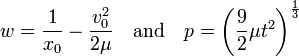
Where t is the time,  is the initial position,
  is the initial velocity, and .
The inverse radial Kepler equation is the solution to the radial Kepler problem:

Evaluating this yields:

Power series can be easily differentiated term by term. Repeated differentiation gives the formulas for the velocity, acceleration, jerk, snap, etc.
Orbit inside a radial shaft
The orbit inside a radial shaft in a uniform spherical body[3] would be a simple harmonic motion, because gravity inside such a body is proportional to the distance to the center. If the small body enters and/or exits the large body at its surface the orbit changes from or to one of those discussed above. For example, if the shaft extends from surface to surface a closed orbit is possible consisting of parts of two cycles of simple harmonic motion and parts of two different (but symmetric) radial elliptic orbits.
See also
References
- Cowell, Peter (1993), Solving Kepler's Equation Over Three Centuries, William Bell.
- ↑ William Tyrrell Thomson (1986), Introduction to Space Dynamics, Dover
- ↑ Brown, Kevin,http://www.mathpages.com/rr/s4-03/4-03.htm, MathPages
- ↑ Strictly this is a contradiction. However, it is assumed that the shaft causes a negligible influence on the gravity.