Segmented regression
| Part of a series on Statistics |
| Regression analysis |
|---|
 |
| Models |
| Estimation |
| Background |
|
Segmented regression, also known as piecewise regression or 'broken-stick regression', is a method in regression analysis in which the independent variable is partitioned into intervals and a separate line segment is fit to each interval. Segmented regression analysis can also be performed on multivariate data by partitioning the various independent variables. Segmented regression is useful when the independent variables, clustered into different groups, exhibit different relationships between the variables in these regions. The boundaries between the segments are breakpoints.
Segmented linear regression is segmented regression whereby the relations in the intervals are obtained by linear regression.
Segmented linear regression, two segments

Segmented linear regression with two segments separated by a breakpoint can be useful to quantify an abrupt change of the response function (Yr) of a varying influential factor (x). The breakpoint can be interpreted as a critical, safe, or threshold value beyond or below which (un)desired effects occur. The breakpoint can be important in decision making [1]
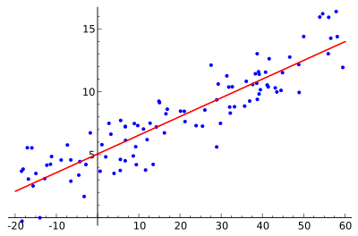
The figures illustrate some of the results and regression types obtainable.
A segmented regression analysis is based on the presence of a set of ( y, x ) data, in which y is the dependent variable and x the independent variable.
The least squares method applied separately to each segment, by which the two regression lines are made to fit the data set as closely as possible while minimizing the sum of squares of the differences (SSD) between observed (y) and calculated (Yr) values of the dependent variable, results in the following two equations:
- Yr = A1.x + K1 for x < BP (breakpoint)
- Yr = A2.x + K2 for x > BP (breakpoint)
where:
- Yr is the expected (predicted) value of y for a certain value of x;
- A1 and A2 are regression coefficients (indicating the slope of the line segments);
- K1 and K2 are regression constants (indicating the intercept at the y-axis).
The data may show many types or trends,[2] see the figures.
The method also yields two correlation coefficients (R):
- for x < BP (breakpoint)

and
- for x > BP (breakpoint)

where:
- is the minimized SSD per segment

and
- Ya1 and Ya2 are the average values of y in the respective segments.
In the determination of the most suitable trend, statistical tests must be performed to ensure that this trend is reliable (significant).
When no significant breakpoint can be detected, one must fall back on a regression without breakpoint.
Example
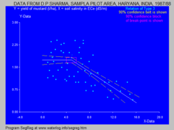
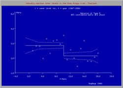
For the blue figure at the right that gives the relation between yield of mustard (Yr = Ym, t/ha) and soil salinity (x = Ss, expressed as electric conductivity of the soil solution EC in dS/m) it is found that:[3]
BP = 4.93, A1 = 0, K1 = 1.74, A2 = −0.129, K2 = 2.38, R12 = 0.0035 (insignificant), R22 = 0.395 (significant) and:
- Ym = 1.74 t/ha for Ss < 4.93 (breakpoint)
- Ym = −0.129 Ss + 2.38 t/ha for Ss > 4.93 (breakpoint)
indicating that soil salinities < 4.93 dS/m are safe and soil salinities > 4.93 dS/m reduce the yield @ 0.129 t/ha per unit increase of soil salinity.
The figure also shows confidence intervals and uncertainty as elaborated hereunder.
Test procedures
The following statistical tests are used to determine the type of trend:
- significance of the breakpoint (BP) by expressing BP as a function of regression coefficients A1 and A2 and the means Y1 and Y2 of the y-data and the means X1 and X2 of the x data (left and right of BP), using the laws of propagation of errors in additions and multiplications to compute the standard error (SE) of BP, and applying Student's t-test
- significance of A1 and A2 applying Student's t-distribution and the standard error SE of A1 and A2
- significance of the difference of A1 and A2 applying Student's t-distribution using the SE of their difference.
- significance of the difference of Y1 and Y2 applying Student's t-distribution using the SE of their difference.
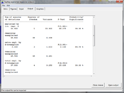
In addition, use is made of the correlation coefficient of all data (Ra), the coefficient of determination or coefficient of explanation, confidence intervals of the regression functions, and Anova analysis.[4]
The coefficient of determination for all data (Cd), that is to be maximized under the conditions set by the significance tests, is found from:

where Yr is the expected (predicted) value of y according to the former regression equations and Ya is the average of all y values.
The Cd coefficient ranges between 0 (no explanation at all) to 1 (full explanation, perfect match).
In a pure, unsegmented, linear regression, the values of Cd and Ra2 are equal. In a segmented regression, Cd needs to be significantly larger than Ra2 to justify the segmentation.
The optimal value of the breakpoint may be found such that the Cd coefficient is maximum.
No-effect range
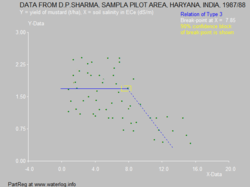
Segmented regression is often used to detect over which range an explanatory variable (X) has no effect on the dependent variable (Y), while beyond the reach there is a clear response, be it positive or negative. The reach of no effect be found at the initial part of X domain or conversely at its last part. For the "no effect" analysis, application of the least squares method for the segmented regression analysis [5] may not be the most appropriate technique because the aim is rather to find the longest stretch over which the Y-X relation can be considered to possess zero slope while beyond the reach the slope is significantly different from zero but knowledge about the best value of this slope is not material. The method to find the no-effect range is progressive partial regression [6] over the range, extending the range with small steps until the regression coefficient gets significantly different from zero.
In the next figure the break point is found at X=7.9 while for the same data (see blue figure above for mustard yield), the least squares method yields a break point only at X=4.9. The latter value is lower, but the fit of the data beyond the break point is better. Hence, it will depend on the purpose of the analysis which method needs to be employed.
See also
- Chow test
- Simple regression
- Linear regression
- Ordinary least squares
- Multivariate adaptive regression splines
- Local regression
- Regression discontinuity design
- Stepwise regression
- SegReg (software) for segmented regression
References
- ↑ Frequency and Regression Analysis. Chapter 6 in: H.P.Ritzema (ed., 1994), Drainage Principles and Applications, Publ. 16, pp. 175-224, International Institute for Land Reclamation and Improvement (ILRI), Wageningen, The Netherlands. ISBN 90-70754-33-9 . Free download from the webpage , under nr. 13, or directly as PDF :
- ↑ Drainage research in farmers' fields: analysis of data. Part of project "Liquid Gold" of the International Institute for Land Reclamation and Improvement (ILRI), Wageningen, The Netherlands. Download as PDF :
- ↑ R.J.Oosterbaan, D.P.Sharma, K.N.Singh and K.V.G.K.Rao, 1990, Crop production and soil salinity: evaluation of field data from India by segmented linear regression. In: Proceedings of the Symposium on Land Drainage for Salinity Control in Arid and Semi-Arid Regions, February 25th to March 2nd, 1990, Cairo, Egypt, Vol. 3, Session V, p. 373 - 383.
- ↑ Statistical significance of segmented linear regression with break-point using variance analysis and F-tests. Download from under nr. 13, or directly as PDF :
- ↑ Segmented regression analysis, International Institute for Land Reclamation and Improvement (ILRI), Wageningen, The Netherlands. Free download from the webpage
- ↑ Partial Regression Analysis, International Institute for Land Reclamation and Improvement (ILRI), Wageningen, The Netherlands. Free download from the webpage