Stackelberg competition

The Stackelberg leadership model is a strategic game in economics in which the leader firm moves first and then the follower firms move sequentially. It is named after the German economist Heinrich Freiherr von Stackelberg who published Market Structure and Equilibrium (Marktform und Gleichgewicht) in 1934 which described the model.

In game theory terms, the players of this game are a leader and a follower and they compete on quantity. The Stackelberg leader is sometimes referred to as the Market Leader.

There are some further constraints upon the sustaining of a Stackelberg equilibrium. The leader must know ex ante that the follower observes its action. The follower must have no means of committing to a future non-Stackelberg follower action and the leader must know this. Indeed, if the 'follower' could commit to a Stackelberg leader action and the 'leader' knew this, the leader's best response would be to play a Stackelberg follower action.

Firms may engage in Stackelberg competition if one has some sort of advantage enabling it to move first. More generally, the leader must have commitment power. Moving observably first is the most obvious means of commitment: once the leader has made its move, it cannot undo it - it is committed to that action. Moving first may be possible if the leader was the incumbent monopoly of the industry and the follower is a new entrant. Holding excess capacity is another means of commitment.

Subgame perfect Nash equilibrium

The Stackelberg model can be solved to find the subgame perfect Nash equilibrium or equilibria (SPNE), i.e. the strategy profile that serves best each player, given the strategies of the other player and that entails every player playing in a Nash equilibrium in every subgame.

In very general terms, let the price function for the (duopoly) industry be $P$; price is simply a function of total (industry) output, so is $P(q_{1}+q_{2})$ where the subscript 1 represents the leader and 2 represents the follower. Suppose firm i has the cost structure $C_{i}(q_{i})$. The model is solved by backward induction. The leader considers what the best response of the follower is, i.e. how it will respond once it has observed the quantity of the leader. The leader then picks a quantity that maximises its payoff, anticipating the predicted response of the follower. The follower actually observes this and in equilibrium picks the expected quantity as a response.

To calculate the SPNE, the best response functions of the follower must first be calculated (calculation moves 'backwards' because of backward induction).

The profit of firm 2 (the follower) is revenue minus cost. Revenue is the product of price and quantity and cost is given by the firm's cost structure, so profit is: $\Pi _{2}=P(q_{1}+q_{2})\cdot q_{2}-C_{2}(q_{2})$. The best response is to find the value of $q_{2}$ that maximises $\Pi _{2}$ given $q_{1}$, i.e. given the output of the leader (firm 1), the output that maximises the follower's profit is found. Hence, the maximum of $\Pi _{2}$ with respect to $q_{2}$ is to be found. First differentiate $\Pi _{2}$ with respect to $q_{2}$:

${\frac {\partial \Pi _{2}}{\partial q_{2}}}={\frac {\partial P(q_{1}+q_{2})}{\partial q_{2}}}\cdot q_{2}+P(q_{1}+q_{2})-{\frac {\partial C_{2}(q_{2})}{\partial q_{2}}}.$

Setting this to zero for maximisation:

${\frac {\partial \Pi _{2}}{\partial q_{2}}}={\frac {\partial P(q_{1}+q_{2})}{\partial q_{2}}}\cdot q_{2}+P(q_{1}+q_{2})-{\frac {\partial C_{2}(q_{2})}{\partial q_{2}}}=0.$

The values of $q_{2}$ that satisfy this equation are the best responses. Now the best response function of the leader is considered. This function is calculated by considering the follower's output as a function of the leader's output, as just computed.

The profit of firm 1 (the leader) is $\Pi _{1}=P(q_{1}+q_{2}(q_{1})).q_{1}-C_{1}(q_{1})$, where $q_{2}(q_{1})$ is the follower's quantity as a function of the leader's quantity, namely the function calculated above. The best response is to find the value of $q_{1}$ that maximises $\Pi _{1}$ given $q_{2}(q_{1})$, i.e. given the best response function of the follower (firm 2), the output that maximises the leader's profit is found. Hence, the maximum of $\Pi _{1}$ with respect to $q_{1}$ is to be found. First, differentiate $\Pi _{1}$ with respect to $q_{1}$:

${\frac {\partial \Pi _{1}}{\partial q_{1}}}={\frac {\partial P(q_{1}+q_{2})}{\partial q_{2}}}\cdot {\frac {\partial q_{2}(q_{1})}{\partial q_{1}}}\cdot q_{1}+{\frac {\partial P(q_{1}+q_{2})}{\partial q_{1}}}\cdot q_{1}+P(q_{1}+q_{2}(q_{1}))-{\frac {\partial C_{1}(q_{1})}{\partial q_{1}}}.$

Setting this to zero for maximisation:

${\frac {\partial \Pi _{1}}{\partial q_{1}}}={\frac {\partial P(q_{1}+q_{2})}{\partial q_{2}}}\cdot {\frac {\partial q_{2}(q_{1})}{\partial q_{1}}}\cdot q_{1}+{\frac {\partial P(q_{1}+q_{2})}{\partial q_{1}}}\cdot q_{1}+P(q_{1}+q_{2}(q_{1}))-{\frac {\partial C_{1}(q_{1})}{\partial q_{1}}}=0.$

Examples

The following example is very general. It assumes a generalised linear demand structure

$P(q_{1}+q_{2})={\bigg (}a-b(q_{1}+q_{2}){\bigg )}$

and imposes some restrictions on cost structures for simplicity's sake so the problem can be resolved.

${\frac {\partial ^{2}C_{i}(q_{i})}{\partial q_{i}\cdot \partial q_{j}}}=0,\forall j$ and ${\frac {\partial C_{i}(q_{i})}{\partial q_{j}}}=0,j\neq \ i$

for ease of computation.

The follower's profit is:

$\Pi _{2}={\bigg (}a-b(q_{1}+q_{2}){\bigg )}\cdot q_{2}-C_{2}(q_{2}).$

The maximisation problem resolves to (from the general case):

${\frac {\partial {\bigg (}a-b(q_{1}+q_{2}){\bigg )}}{\partial q_{2}}}\cdot q_{2}+a-b(q_{1}+q_{2})-{\frac {\partial C_{2}(q_{2})}{\partial q_{2}}}=0,$

$\Rightarrow \ -bq_{2}+a-b(q_{1}+q_{2})-{\frac {\partial C_{2}(q_{2})}{\partial q_{2}}}=0,$

$\Rightarrow \ q_{2}={\frac {a-bq_{1}-{\frac {\partial C_{2}(q_{2})}{\partial q_{2}}}}{2b}}.$

Consider the leader's problem:

$\Pi _{1}={\bigg (}a-b(q_{1}+q_{2}(q_{1})){\bigg )}\cdot q_{1}-C_{1}(q_{1}).$

Substituting for $q_{2}(q_{1})$ from the follower's problem:

$\Pi _{1}={\bigg (}a-b{\bigg (}q_{1}+{\frac {a-bq_{1}-{\frac {\partial C_{2}(q_{2})}{\partial q_{2}}}}{2b}}{\bigg )}{\bigg )}\cdot q_{1}-C_{1}(q_{1}),$

$\Rightarrow \Pi _{1}={\bigg (}{\frac {a-b.q_{1}+{\frac {\partial C_{2}(q_{2})}{\partial q_{2}}}}{2}}){\bigg )}\cdot q_{1}-C_{1}(q_{1}).$

The maximisation problem resolves to (from the general case):

${\frac {\partial \Pi _{1}}{\partial q_{1}}}={\bigg (}{\frac {a-2bq_{1}+{\frac {\partial C_{2}(q_{2})}{\partial q_{2}}}}{2}}{\bigg )}-{\frac {\partial C_{1}(q_{1})}{\partial q_{1}}}=0.$

Now solving for $q_{1}$ yields $q_{1}^{*}$, the leader's optimal action:

$q_{1}^{*}={\frac {a+{\frac {\partial C_{2}(q_{2})}{\partial q_{2}}}-2\cdot {\frac {\partial C_{1}(q_{1})}{\partial q_{1}}}}{2b}}.$

This is the leader's best response to the reaction of the follower in equilibrium. The follower's actual can now be found by feeding this into its reaction function calculated earlier:

$q_{2}^{*}={\frac {a-b\cdot {\frac {a+{\frac {\partial C_{2}(q_{2})}{\partial q_{2}}}-2\cdot {\frac {\partial C_{1}(q_{1})}{\partial q_{1}}}}{2b}}-{\frac {\partial C_{2}(q_{2})}{\partial q_{2}}}}{2b}},$

$\Rightarrow q_{2}^{*}={\frac {a-3\cdot {\frac {\partial C_{2}(q_{2})}{\partial q_{2}}}+2\cdot {\frac {\partial C_{1}(q_{1})}{\partial q_{1}}}}{4b}}.$

The Nash equilibria are all $(q_{1}^{*},q_{2}^{*})$. It is clear (if marginal costs are assumed to be zero - i.e. cost is essentially ignored) that the leader has a significant advantage. Intuitively, if the leader was no better off than the follower, it would simply adopt a Cournot competition strategy.

Plugging the follower's quantity $q_{2}$, back into the leader's best response function will not yield $q_{1}$. This is because once leader has committed to an output and observed the followers it always wants to reduce its output ex-post. However its inability to do so is what allows it to receive higher profits than under cournot.

Economic analysis

An extensive-form representation is often used to analyze the Stackelberg leader-follower model. Also referred to as a “decision tree”, the model shows the combination of outputs and payoffs both firms have in the Stackelberg game

A Stackelberg game represented in extensive form

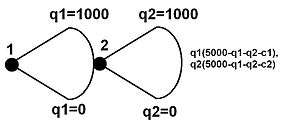
The image on the left depicts in extensive form a Stackelberg game. The payoffs are shown on the right. This example is fairly simple. There is a basic cost structure involving only marginal cost (there is no fixed cost). The demand function is linear and price elasticity of demand is 1. However, it illustrates the leader's advantage.

The follower wants to choose $q_{2}$ to maximise its payoff $q_{2}*(5000-q_{1}-q_{2}-c_{2})$. Taking the first order derivative and equating it to zero (for maximisation) yields $q_{2}={\frac {5000-q_{1}-c_{2}}{2}}$ as the maximum value of $q_{2}$.

The leader wants to choose $q_{1}$ to maximise its payoff $q_{1}*(5000-q_{1}-q_{2}-c_{1})$. However, in equilibrium, it knows the follower will choose $q_{2}$ as above. So in fact the leader wants to maximise its payoff $q_{1}*(5000-q_{1}-{\frac {5000-q_{1}-c_{2}}{2}}-c_{1})$ (by substituting $q_{2}$ for the follower's best response function). By differentiation, the maximum payoff is given by $q_{1}={\frac {5000-2c_{1}+c_{2}}{2}}$. Feeding this into the follower's best response function yields $q_{2}={\frac {5000+2c_{1}-3c_{2}}{4}}$. Suppose marginal costs were equal for the firms (so the leader has no market advantage other than first move) and in particular $c_{1}=c_{2}=1000$. The leader would produce 2000 and the follower would produce 1000. This would give the leader a profit (payoff) of two million and the follower a profit of one million. Simply by moving first, the leader has accrued twice the profit of the follower. However, Cournot profits here are 1.78 million apiece (strictly, $(16/9)10^{{6}}$ apiece), so the leader has not gained much, but the follower has lost. However, this is example-specific. There may be cases where a Stackelberg leader has huge gains beyond Cournot profit that approach monopoly profits (for example, if the leader also had a large cost structure advantage, perhaps due to a better production function). There may also be cases where the follower actually enjoys higher profits than the leader, but only because it, say, has much lower costs. This behaviour consistently work on duopoly markets even if the firms are assymetrical.

Credible and non-credible threats by the follower

If, after the leader had selected its equilibrium quantity, the follower deviated from the equilibrium and chose some non-optimal quantity it would not only hurt itself, but it could also hurt the leader. If the follower chose a much larger quantity than its best response, the market price would lower and the leader's profits would be stung, perhaps below Cournot level profits. In this case, the follower could announce to the leader before the game starts that unless the leader chooses a Cournot equilibrium quantity, the follower will choose a deviant quantity that will hit the leader's profits. After all, the quantity chosen by the leader in equilibrium is only optimal if the follower also plays in equilibrium. The leader is, however, in no danger. Once the leader has chosen its equilibrium quantity, it would be irrational for the follower to deviate because it too would be hurt. Once the leader has chosen, the follower is better off by playing on the equilibrium path. Hence, such a threat by the follower would not be credible.

However, in an (indefinitely) repeated Stackelberg game, the follower might adopt a punishment strategy where it threatens to punish the leader in the next period unless it chooses a non-optimal strategy in the current period. This threat may be credible because it could be rational for the follower to punish in the next period so that the leader chooses Cournot quantities thereafter.

Stackelberg compared with Cournot

The Stackelberg and Cournot models are similar because in both competition is on quantity. However, as seen, the first move gives the leader in Stackelberg a crucial advantage. There is also the important assumption of perfect information in the Stackelberg game: the follower must observe the quantity chosen by the leader, otherwise the game reduces to Cournot. With imperfect information, the threats described above can be credible. If the follower cannot observe the leader's move, it is no longer irrational for the follower to choose, say, a Cournot level of quantity (in fact, that is the equilibrium action). However, it must be that there is imperfect information and the follower is unable to observe the leader's move because it is irrational for the follower not to observe if it can once the leader has moved. If it can observe, it will so that it can make the optimal decision. Any threat by the follower claiming that it will not observe even if it can is as uncredible as those above. This is an example of too much information hurting a player. In Cournot competition, it is the simultaneity of the game (the imperfection of knowledge) that results in neither player (ceteris paribus) being at a disadvantage.

Game theoretic considerations

As mentioned, imperfect information in a leadership game reduces to Cournot competition. However, some Cournot strategy profiles are sustained as Nash equilibria but can be eliminated as incredible threats (as described above) by applying the solution concept of subgame perfection. Indeed, it is the very thing that makes a Cournot strategy profile a Nash equilibrium in a Stackelberg game that prevents it from being subgame perfect.

Consider a Stackelberg game (i.e. one which fulfills the requirements described above for sustaining a Stackelberg equilibrium) in which, for some reason, the leader believes that whatever action it takes, the follower will choose a Cournot quantity (perhaps the leader believes that the follower is irrational). If the leader played a Stackelberg action, (it believes) that the follower will play Cournot. Hence it is non-optimal for the leader to play Stackelberg. In fact, its best response (by the definition of Cournot equilibrium) is to play Cournot quantity. Once it has done this, the best response of the follower is to play Cournot.

Consider the following strategy profiles: the leader plays Cournot; the follower plays Cournot if the leader plays Cournot and the follower plays non-Stackelberg if the leader plays Stackelberg and if the leader plays something else, the follower plays an arbitrary strategy (hence this actually describes several profiles). This profile is a Nash equilibrium. As argued above, on the equilibrium path play is a best response to a best response. However, playing Cournot would not have been the best response of the leader were it that the follower would play Stackelberg if it (the leader) played Stackelberg. In this case, the best response of the leader would be to play Stackelberg. Hence, what makes this profile (or rather, these profiles) a Nash equilibrium (or rather, Nash equilibria) is the fact that the follower would play non-Stackelberg if the leader were to play Stackelberg.

However, this very fact (that the follower would play non-Stackelberg if the leader were to play Stackelberg) means that this profile is not a Nash equilibrium of the subgame starting when the leader has already played Stackelberg (a subgame off the equilibrium path). If the leader has already played Stackelberg, the best response of the follower is to play Stackelberg (and therefore it is the only action that yields a Nash equilibrium in this subgame). Hence the strategy profile - which is Cournot - is not subgame perfect.

Comparison with other oligopoly models

In comparison with other oligopoly models,

• The aggregate Stackelberg output is greater than the aggregate Cournot output, but less than the aggregate Bertrand output.
• The Stackelberg price is lower than the Cournot price, but greater than the Bertrand price.
• The Stackelberg consumer surplus is greater than the Cournot consumer surplus, but lower than the Bertrand consumer surplus.
• The aggregate Stackelberg output is greater than pure monopoly or cartel, but less than the perfectly competitive output.
• The Stackelberg price is lower than the pure monopoly or cartel price, but greater than the perfectly competitive price.

Applications

The Stackelberg concept has been extended to dynamic Stackelberg games. See Simaan and Cruz (1973a, 1973b). With the addition of time as a dimension, phenomena not found in static games were discovered, such as violation of the principle of optimality by the leader, Simaan and Cruz (1973b). For a survey of applications of Stackelberg differential games to supply chain and marketing channels, see He et al. (2007). In recent years, Stackelberg games have contributed a lot in the security domain^[1] where it is essential for the security personnel to protect some valuable resource and search for any potential threats to it. This is where it involves the security personnel (leader) to design his/her strategy first so that irrespective of the strategy adopted by the thief (follower), the resource remains safe.

See also

• Economic theory
• Cournot competition
• Bertrand competition
• Extensive form game
• Industrial organization
• Mathematical programming with equilibrium constraints

References

1. Brown, Gerald (2006). "Defending critical infrastructure". Interfaces. 36 (6): 530–544.

• H. von Stackelberg, Market Structure and Equilibrium: 1st Edition Translation into English, Bazin, Urch & Hill, Springer 2011, XIV, 134 p., ISBN 978-3-642-12585-0
• M. Simaan and J.B. Cruz, Jr., On the Stackelberg Strategy in Nonzero-Sum Games, Journal of Optimization Theory and Applications, Vol. 11, No. 5, May 1973, pp. 533–555.
• M. Simaan and J.B. Cruz, Jr., Additional Aspects of the Stackelberg Strategy in Nonzero-Sum Games, Journal of Optimization Theory and Applications, Vol. 11, No. 6, June 1973, pp. 613–626.
• He, X., Prasad, A., Sethi, S.P., and Gutierrez, G. (2007) A Survey of Stackelberg Differential Game Models in Supply and Marketing Channels, Journal of Systems Science and Systems Engineering (JSSSE), 16(4), December 2007, 385-413. Available at http://papers.ssrn.com/sol3/papers.cfm?abstract_id=1069162
• Fudenberg, D. and Tirole, J. (1993) Game Theory, MIT Press. (see Chapter 3, sect 1)
• Gibbons, R. (1992) A primer in game theory, Harvester-Wheatsheaf. (see Chapter 2, section 1B)
• Osborne, M.J. and Rubenstein, A. (1994) A Course in Game Theory, MIT Press (see p 97-98)
• Oligoply Theory made Simple, Chapter 6 of Surfing Economics by Huw Dixon.