Time-invariant system
A time-invariant (TIV) system is a system whose output does not depend explicitly on time. Such systems are regarded as a class of systems in the field of system analysis. Lack of time dependence is captured in the following mathematical property of such a system:
- If the input signal
 produces an output
  then any time shifted input,
  , results in a time-shifted output
This property can be satisfied if the transfer function of the system is not a function of time except expressed by the input and output.
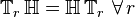
In the context of a system schematic, this property can also be stated as follows:
- If a system is time-invariant then the system block commutes with an arbitrary delay.
If a time-invariant system is also linear, it is the subject of LTI system theory (linear time-invariant) with direct applications in NMR spectroscopy, seismology, circuits, signal processing, control theory, and other technical areas. Nonlinear time-invariant systems lack a comprehensive, governing theory. Discrete time-invariant systems are known as shift-invariant systems. Systems which lack the time-invariant property are studied as time-variant systems.
Simple example
To demonstrate how to determine if a system is time-invariant, consider the two systems:
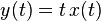
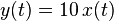
- System A:
- System B:
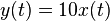
Since system A explicitly depends on t outside of and , it is not time-invariant. System B, however, does not depend explicitly on t so it is time-invariant.
Formal example
A more formal proof of why systems A and B above differ is now presented. To perform this proof, the second definition will be used.
System A:
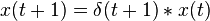
- Start with a delay of the input
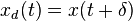
- Now delay the output by

- Clearly
 , therefore the system is not time-invariant.


System B:
- Start with a delay of the input
- Now delay the output by

- Clearly
 , therefore the system is time-invariant.


Abstract example
We can denote the shift operator by  where
where  is the amount by which a vector's index set should be shifted. For example, the "advance-by-1" system
can be represented in this abstract notation by

where  is a function given by
with the system yielding the shifted output
So  is an operator that advances the input vector by 1.
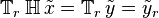
Suppose we represent a system by an operator  . This system is time-invariant if it commutes with the shift operator, i.e.,
If our system equation is given by

then it is time-invariant if we can apply the system operator on followed by the shift operator , or we can apply the shift operator followed by the system operator , with the two computations yielding equivalent results.
Applying the system operator first gives
Applying the shift operator first gives
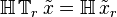
If the system is time-invariant, then
