Unimodality
In mathematics, unimodality means possessing a unique mode. More generally, unimodality means there is only a single highest value, somehow defined, of some mathematical object.[1]
Unimodal probability distribution


In statistics, a unimodal probability distribution (or when referring to the distribution, a unimodal distribution) is a probability distribution which has a single mode. As the term "mode" has multiple meanings, so does the term "unimodal".
Strictly speaking, a mode of a discrete probability distribution is a value at which the probability mass function (pmf) takes its maximum value. In other words, it is a most likely value. A mode of a continuous probability distribution is a value at which the probability density function (pdf) attains its maximum value. Note that in both cases there can be more than one mode, since the maximum value of either the pmf or the pdf can be attained at more than one value.
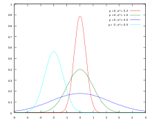
If there is a single mode, the distribution function is called "unimodal". If it has more modes it is "bimodal" (2), "trimodal" (3), etc., or in general, "multimodal".[2] Figure 1 illustrates normal distributions, which are unimodal. Other examples of unimodal distributions include Cauchy distribution, Student's t-distribution, chi-squared distribution and exponential distribution. Among discrete distributions, the binomial distribution and Poisson distribution can be seen as unimodal, though for some parameters they can have two adjacent values with the same probability.
Figure 2 illustrates a bimodal distribution.
Figure 3 illustrates a distribution with a single global maximum which by strict definition is unimodal. However, confusingly, and mostly with continuous distributions, when a pdf function has multiple local maxima it is common to refer to all of the local maxima as modes of the distribution. Therefore, if a pdf has more than one local maximum it is referred to as multimodal. Under this common definition, Figure 3 illustrates a bimodal distribution.
Other definitions
Other definitions of unimodality in distribution functions also exist.
In continuous distributions, unimodality can be defined through the behavior of the cumulative distribution function (cdf).[3] If the cdf is convex for x < m and concave for x > m, then the distribution is unimodal, m being the mode. Note that under this definition the uniform distribution is unimodal,[4] as well as any other distribution in which the maximum distribution is achieved for a range of values, e.g. trapezoidal distribution. Note also that usually this definition allows for a discontinuity at the mode; usually in a continuous distribution the probability of any single value is zero, while this definition allows for a non-zero probability, or an "atom of probability", at the mode.
Criteria for unimodality can also be defined through the characteristic function of the distribution[3] or through its Laplace–Stieltjes transform.[5]
Another way to define a unimodal discrete distribution is by the occurrence of sign changes in the sequence of differences of the probabilities.[6] A discrete distribution with a probability mass function, , is called unimodal if the sequence has exactly one sign change (when zeroes don't count).


Uses and results
One reason for the importance of distribution unimodality is that it allows for several important results. Several Inequalities are given below which are only valid for unimodal distributions. Thus, it is important to assess whether or not a given data set comes from a unimodal distribution. Several tests for unimodality are given in the Wiki article on Multimodal Distribution
Inequalities
Gauss' inequality
A first important result is Gauss's inequality.[7] Gauss's inequality gives an upper bound on the probability that a value lies more than any given distance from its mode. This inequality depends on unimodality.
Vysochanskiï–Petunin inequality
A second is the Vysochanskiï–Petunin inequality,[8] a refinement of the Chebyshev inequality. The Chebyshev inequality guarantees that in any probability distribution, "nearly all" the values are "close to" the mean value. The Vysochanskiï–Petunin inequality refines this to even nearer values, provided that the distribution function is continuous and unimodal. Further results were shown by Sellke & Sellke.[9]
Mode, median and mean
Gauss also showed in 1823 that for a unimodal distribution[10]

and

where the median is ν, the mean is μ and ω is the root mean square deviation from the mode.
It can be shown for a unimodal distribution that the median ν and the mean μ lie within (3/5)1/2 ≈ 0.7746 standard deviations of each other.[11] In symbols,

where |.| is the absolute value.
A similar relation holds between the median and the mode θ: they lie within 31/2 ≈ 1.732 standard deviations of each other:

It can also be shown that the mean and the mode lie within 31/2 of each other.

Skewness and kurtosis
Rohatgi and Szekely have shown that the skewness and kurtosis of a unimodal distribution are related by the inequality:[12]

where κ is the kurtosis and γ is the skewness.
Klaassen, Mokveld, and van Es derived a slightly different inequality (shown below) from the one derived by Rohatgi and Szekely (shown above), which tends to be more inclusive (i.e., yield more positives) in tests of unimodality:[13]

Unimodal function
As the term "modal" applies to data sets and probability distribution, and not in general to functions, the definitions above do not apply. The definition of "unimodal" was extended to functions of real numbers as well.
A common definition is as follows: a function f(x) is a unimodal function if for some value m, it is monotonically increasing for x ≤ m and monotonically decreasing for x ≥ m. In that case, the maximum value of f(x) is f(m) and there are no other local maxima.
Proving unimodality is often hard. One way consists in using the definition of that property, but it turns out to be suitable for simple functions only. A general method based on derivatives exists,[14] but it does not succeed for every function despite its simplicity.
Examples of unimodal functions include quadratic polynomial functions with a negative quadratic coefficient, tent map functions, and more.
The above is sometimes related to as "strong unimodality", from the fact that the monotonicity implied is strong monotonicity. A function f(x) is a weakly unimodal function if there exists a value m for which it is weakly monotonically increasing for x ≤ m and weakly monotonically decreasing for x ≥ m. In that case, the maximum value f(m) can be reached for a continuous range of values of x. An example of a weakly unimodal function which is not strongly unimodal is every other row in a Pascal triangle.
Depending on context, unimodal function may also refer to a function that has only one local minimum, rather than maximum.[15] For example, local unimodal sampling, a method for doing numerical optimization, is often demonstrated with such a function. It can be said that a unimodal function under this extension is a function with a single local extremum.
One important property of unimodal functions is that the extremum can be found using search algorithms such as golden section search, ternary search or successive parabolic interpolation.
Other extensions
A function f(x) is "S-unimodal" (often referred to as "S-unimodal map") if its Schwarzian derivative is negative for all , where is the critical point.[16]


In computational geometry if a function is unimodal it permits the design of efficient algorithms for finding the extrema of the function.[17]
A more general definition, applicable to a function f(X) of a vector variable X is that f is unimodal if there is a one-to-one differentiable mapping X = G(Z) such that f(G(Z)) is convex. Usually one would want G(Z) to be continuously differentiable with nonsingular Jacobian matrix.
Quasiconvex functions and quasiconcave functions extend the concept of unimodality to functions whose arguments belong to higher-dimensional Euclidean spaces.
See also
References
- ↑ Weisstein, Eric W. "Unimodal". MathWorld.
- ↑ Weisstein, Eric W. "Mode". MathWorld.
- 1 2 A.Ya. Khinchin (1938). "On unimodal distributions". Trams. Res. Inst. Math. Mech. (in Russian). University of Tomsk. 2 (2): 1–7.
- ↑ Ushakov, N.G. (2001), "Unimodal distribution", in Hazewinkel, Michiel, Encyclopedia of Mathematics, Springer, ISBN 978-1-55608-010-4
- ↑ Vladimirovich Gnedenko and Victor Yu Korolev (1996). Random summation: limit theorems and applications. CRC-Press. ISBN 0-8493-2875-6. p. 31
- ↑ Medgyessy, P. (March 1972). "On the unimodality of discrete distributions". Periodica Mathematica Hungarica. 2 (1–4): 245–257. doi:10.1007/bf02018665.
- ↑ Gauss, C. F. (1823). "Theoria Combinationis Observationum Erroribus Minimis Obnoxiae, Pars Prior". Commentationes Societatis Regiae Scientiarum Gottingensis Recentiores. 5.
- ↑ D. F. Vysochanskij, Y. I. Petunin (1980). "Justification of the 3σ rule for unimodal distributions". Theory of Probability and Mathematical Statistics. 21: 25–36.
- ↑ Sellke, T.M.; Sellke, S.H. (1997). "Chebyshev inequalities for unimodal distributions". American Statistician. American Statistical Association. 51 (1): 34–40. doi:10.2307/2684690. JSTOR 2684690.
- ↑ Gauss C.F. Theoria Combinationis Observationum Erroribus Minimis Obnoxiae. Pars Prior. Pars Posterior. Supplementum. Theory of the Combination of Observations Least Subject to Errors. Part One. Part Two. Supplement. 1995. Translated by G.W. Stewart. Classics in Applied Mathematics Series, Society for Industrial and Applied Mathematics, Philadelphia
- ↑ Basu, Sanjib, and Anirban DasGupta. "The mean, median, and mode of unimodal distributions: a characterization." Theory of Probability & Its Applications 41.2 (1997): 210-223.
- ↑ Rohatgi VK, Szekely GJ (1989) Sharp inequalities between skewness and kurtosis. Statistics & Probability Letters 8:297-299
- ↑ Klaassen CAJ, Mokveld PJ, van Es B (2000) Squared skewness minus kurtosis bounded by 186/125 for unimodal distributions. Stat & Prob Lett 50 (2) 131–135
- ↑ "On the unimodality of METRIC Approximation subject to normally distributed demands." (PDF). Method in appendix D, Example in theorem 2 page 5. Retrieved 2013-08-28.
- ↑ "Mathematical Programming Glossary.". Retrieved 2010-07-07.
- ↑ See e.g. John Guckenheimer and Stewart Johnson (July 1990). "Distortion of S-Unimodal Maps". The Annals of Mathematics, Second Series. 132 (1). pp. 71–130. doi:10.2307/1971501.
- ↑ Godfried T. Toussaint (June 1984). "Complexity, convexity, and unimodality". International Journal of Computer and Information Sciences. 13 (3). pp. 197–217. doi:10.1007/bf00979872.