Chi-squared distribution

chi-squared

Probability density function
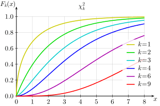
Cumulative distribution function
Notation	$\chi ^{2}(k)\!$ or $\chi _{k}^{2}\!$
Parameters	$k\in \mathbb {N} _{>0}~~$ (known as "degrees of freedom")
Support	x ∈ [0, +∞)
PDF	${\frac {1}{2^{\frac {k}{2}}\Gamma \left({\frac {k}{2}}\right)}}\;x^{{\frac {k}{2}}-1}e^{-{\frac {x}{2}}}\,$
CDF	${\displaystyle {\frac {1}{\Gamma \left({\frac {k}{2}}\right)}}\;\gamma \left({\tfrac {k}{2}},\,{\frac {x}{2}}\right)}$
Mean	k
Median	$\approx k{\bigg (}1-{\frac {2}{9k}}{\bigg )}^{3}$
Mode	max{ k − 2, 0 }
Variance	2k
Skewness	$\scriptstyle {\sqrt {8/k}}\,$
Ex. kurtosis	12 / k
Entropy	${\displaystyle {\begin{aligned}{\tfrac {k}{2}}&+\ln(2\Gamma ({\tfrac {k}{2}}))\\&\!+(1-{\tfrac {k}{2}})\psi ({\tfrac {k}{2}})\,{\scriptstyle {\text{(nats)}}}\end{aligned}}}$
MGF	(1 − 2 t )^−k/2   for t < ½
CF	(1 − 2 i t )^−k/2      [1]

In probability theory and statistics, the chi-squared distribution (also chi-square or χ²-distribution) with k degrees of freedom is the distribution of a sum of the squares of k independent standard normal random variables. It is a special case of the gamma distribution and is one of the most widely used probability distributions in inferential statistics, e.g., in hypothesis testing or in construction of confidence intervals.^[2][3][4][5] When it is being distinguished from the more general noncentral chi-squared distribution, this distribution is sometimes called the central chi-squared distribution.

The chi-squared distribution is used in the common chi-squared tests for goodness of fit of an observed distribution to a theoretical one, the independence of two criteria of classification of qualitative data, and in confidence interval estimation for a population standard deviation of a normal distribution from a sample standard deviation. Many other statistical tests also use this distribution, like Friedman's analysis of variance by ranks.

Definition

If Z₁, ..., Z_k are independent, standard normal random variables, then the sum of their squares,

$Q\ =\sum _{i=1}^{k}Z_{i}^{2},$

is distributed according to the chi-squared distribution with k degrees of freedom. This is usually denoted as

$Q\ \sim \ \chi ^{2}(k)\ \ {\text{or}}\ \ Q\ \sim \ \chi _{k}^{2}.$

The chi-squared distribution has one parameter: k — a positive integer that specifies the number of degrees of freedom (i.e. the number of Z_i’s)

Introduction

The chi-squared distribution is used primarily in hypothesis testing. Unlike more widely known distributions such as the normal distribution and the exponential distribution, the chi-squared distribution is rarely used to model natural phenomena. It arises in the following hypothesis tests, among others.

• Chi-squared test of independence in contingency tables
• Chi-squared test of goodness of fit of observed data to hypothetical distributions
• Likelihood-ratio test for nested models
• Log-rank test in survival analysis
• Cochran–Mantel–Haenszel test for stratified contingency tables

It is also a component of the definition of the t-distribution and the F-distribution used in t-tests, analysis of variance, and regression analysis.

The primary reason that the chi-squared distribution is used extensively in hypothesis testing is its relationship to the normal distribution. Many hypothesis tests use a test statistic, such as the t statistic in a t-test. For these hypothesis tests, as the sample size, n, increases, the sampling distribution of the test statistic approaches the normal distribution (Central Limit Theorem). Because the test statistic (such as t) is asymptotically normally distributed, provided the sample size is sufficiently large, the distribution used for hypothesis testing may be approximated by a normal distribution. Testing hypotheses using a normal distribution is well understood and relatively easy. The simplest chi-squared distribution is the square of a standard normal distribution. So wherever a normal distribution could be used for a hypothesis test, a chi-squared distribution could be used.

Specifically, suppose that Z is a standard normal random variable, with mean = 0 and variance = 1. Z ~ N(0,1). A sample drawn at random from Z is a sample from the distribution shown in the graph of the standard normal distribution. Define a new random variable Q. To generate a random sample from Q, take a sample from Z and square the value. The distribution of the squared values is given by the random variable Q = Z². The distribution of the random variable Q is an example of a chi-squared distribution: $\ Q\ \sim \ \chi _{1}^{2}.$ The subscript 1 indicates that this particular chi-squared distribution is constructed from only 1 standard normal distribution. A chi-squared distribution constructed by squaring a single standard normal distribution is said to have 1 degree of freedom. Thus, as the sample size for a hypothesis test increases, the distribution of the test statistic approaches a normal distribution, and the distribution of the square of the test statistic approaches a chi-squared distribution. Just as extreme values of the normal distribution have low probability (and give small p-values), extreme values of the chi-squared distribution have low probability.

An additional reason that the chi-squared distribution is widely used is that it is a member of the class of likelihood ratio tests (LRT).^[6] LRT's have several desirable properties; in particular, LRT's commonly provide the highest power to reject the null hypothesis (Neyman–Pearson lemma). However, the normal and chi-squared approximations are only valid asymptotically. For this reason, it is preferable to use the t distribution rather than the normal approximation or the chi-squared approximation for small sample size. Similarly, in analyses of contingency tables, the chi-squared approximation will be poor for small sample size, and it is preferable to use Fisher's exact test. Ramsey and Ramsey show that the exact binomial test is always more powerful than the normal approximation.^[7]

Lancaster^[8] shows the connections among the binomial, normal, and chi-squared distributions, as follows. De Moivre and Laplace established that a binomial distribution could be approximated by a normal distribution. Specifically they showed the asymptotic normality of the random variable

${\displaystyle \chi ={m-Np \over {\sqrt {(Npq)}}}}$

where m is the observed number of successes in N trials, where the probability of success is p, and q = 1 − p.

Squaring both sides of the equation gives

$\chi ^{2}={(m-Np)^{2} \over (Npq)}$

Using N = Np + N(1 − p), N = m + (N − m), and q = 1 − p, this equation simplifies to

$\chi ^{2}={(m-Np)^{2} \over (Np)}+{(N-m-Nq)^{2} \over (Nq)}$

The expression on the right is of the form that Pearson would generalize to the form:

${\displaystyle \chi ^{2}=\sum _{i=1}^{n}{\frac {(O_{i}-E_{i})^{2}}{E_{i}}}}$

where

$\chi ^{2}$ = Pearson's cumulative test statistic, which asymptotically approaches a $\chi ^{2}$ distribution.

$O_{i}$ = the number of observations of type i.

$E_{i}=Np_{i}$ = the expected (theoretical) frequency of type i, asserted by the null hypothesis that the fraction of type i in the population is $p_{i}$

$n$ = the number of cells in the table.

In the case of a binomial outcome (flipping a coin), the binomial distribution may be approximated by a normal distribution (for sufficiently large n). Because the square of a standard normal distribution is the chi-squared distribution with one degree of freedom, the probability of a result such as 1 heads in 10 trials can be approximated either by the normal or the chi-squared distribution. However, many problems involve more than the two possible outcomes of a binomial, and instead require 3 or more categories, which leads to the multinomial distribution. Just as de Moivre and Laplace sought for and found the normal approximation to the binomial, Pearson sought for and found a multivariate normal approximation to the multinomial distribution. Pearson showed that the chi-squared distribution, the sum of multiple normal distributions, was such an approximation to the multinomial distribution ^[8]

Characteristics

Further properties of the chi-squared distribution can be found in the box at the upper right corner of this article.

Probability density function

The probability density function (pdf) of the chi-square distribution is

${\displaystyle f(x;\,k)={\begin{cases}{\dfrac {x^{(k/2-1)}e^{-x/2}}{2^{k/2}\Gamma \left({\frac {k}{2}}\right)}},&x>0;\\0,&{\text{otherwise}}.\end{cases}}}$

where Γ(k/2) denotes the Gamma function, which has closed-form values for integer k.

For derivations of the pdf in the cases of one, two and k degrees of freedom, see Proofs related to chi-squared distribution.

Differential equation

The pdf of the chi-squared distribution is a solution to the following differential equation:

${\displaystyle 2xf'(x)+f(x)(-k+x+2)=0,}$

with the initial condition:

${\displaystyle f(1)={\frac {2^{-{\frac {k}{2}}}}{{\sqrt {e}}\Gamma \left({\frac {k}{2}}\right)}}.}$

Cumulative distribution function

Chernoff bound for the CDF and tail (1-CDF) of a chi-squared random variable with ten degrees of freedom (k = 10)

Its cumulative distribution function is:

$F(x;\,k)={\frac {\gamma ({\frac {k}{2}},\,{\frac {x}{2}})}{\Gamma ({\frac {k}{2}})}}=P\left({\frac {k}{2}},\,{\frac {x}{2}}\right),$

where γ(s,t) is the lower incomplete Gamma function and P(s,t) is the regularized Gamma function.

In a special case of k = 2 this function has a simple form:

${\displaystyle F(x;\,2)=1-e^{-x/2}}$

and the form is not much more complicated for other small even k .

Tables of the chi-squared cumulative distribution function are widely available and the function is included in many spreadsheets and all statistical packages.

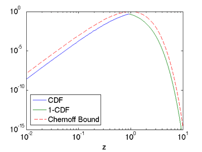
Letting $z\equiv x/k$, Chernoff bounds on the lower and upper tails of the CDF may be obtained.^[9] For the cases when $0<z<1$ (which include all of the cases when this CDF is less than half):

$F(zk;\,k)\leq (ze^{1-z})^{k/2}.$

The tail bound for the cases when $z>1$, similarly, is

$1-F(zk;\,k)\leq (ze^{1-z})^{k/2}.$

For another approximation for the CDF modeled after the cube of a Gaussian, see under Noncentral chi-squared distribution.

Additivity

It follows from the definition of the chi-squared distribution that the sum of independent chi-squared variables is also chi-squared distributed. Specifically, if {X_i}_i=1ⁿ are independent chi-squared variables with {k_i}_i=1ⁿ degrees of freedom, respectively, then Y = X₁ + ⋯ + X_n is chi-squared distributed with k₁ + ⋯ + k_n degrees of freedom.

Sample mean

The sample mean of $n$ i.i.d. chi-squared variables of degree $k$ is distributed according to a gamma distribution with shape $\alpha$ and scale $\theta$ parameters:

${\displaystyle {\bar {X}}={\frac {1}{n}}\sum _{i=1}^{n}X_{i}\sim \operatorname {Gamma} \left(\alpha =n\,k/2,\theta =2/n\right)\qquad {\text{where }}X_{i}\sim \chi ^{2}(k)}$

Asymptotically, given that for a scale parameter $\alpha$ going to infinity, a Gamma distribution converges towards a normal distribution with expectation $\mu =\alpha \cdot \theta$ and variance $\sigma ^{2}=\alpha \,\theta ^{2}$, the sample mean converges towards:

${\bar {X}}{\xrightarrow {n\to \infty }}N(\mu =k,\sigma ^{2}=2\,k/n)$

Note that we would have obtained the same result invoking instead the central limit theorem, noting that for each chi-squared variable of degree $k$ the expectation is $k$ , and its variance $2\,k$ (and hence the variance of the sample mean ${\bar {X}}$ being $\sigma ^{2}=2\,k/n$).

Entropy

The differential entropy is given by

${\displaystyle h=\int _{-\infty }^{\infty }f(x;\,k)\ln f(x;\,k)\,dx={\frac {k}{2}}+\ln \left[2\,\Gamma \left({\frac {k}{2}}\right)\right]+\left(1-{\frac {k}{2}}\right)\,\psi \!\left[{\frac {k}{2}}\right],}$

where ψ(x) is the Digamma function.

The chi-squared distribution is the maximum entropy probability distribution for a random variate X for which ${\displaystyle \operatorname {E} (X)=k}$ and ${\displaystyle \operatorname {E} (\ln(X))=\psi (k/2)+\ln(2)}$ are fixed. Since the chi-squared is in the family of gamma distributions, this can be derived by substituting appropriate values in the Expectation of the Log moment of Gamma. For derivation from more basic principles, see the derivation in moment generating function of the sufficient statistic.

Noncentral moments

The moments about zero of a chi-squared distribution with k degrees of freedom are given by^[10][11]

$\operatorname {E} (X^{m})=k(k+2)(k+4)\cdots (k+2m-2)=2^{m}{\frac {\Gamma (m+{\frac {k}{2}})}{\Gamma ({\frac {k}{2}})}}.$

Cumulants

The cumulants are readily obtained by a (formal) power series expansion of the logarithm of the characteristic function:

$\kappa _{n}=2^{n-1}(n-1)!\,k$

Asymptotic properties

By the central limit theorem, because the chi-squared distribution is the sum of k independent random variables with finite mean and variance, it converges to a normal distribution for large k. For many practical purposes, for k > 50 the distribution is sufficiently close to a normal distribution for the difference to be ignored.^[12] Specifically, if X ~ χ²(k), then as k tends to infinity, the distribution of $(X-k)/{\sqrt {2k}}$ tends to a standard normal distribution. However, convergence is slow as the skewness is ${\sqrt {8/k}}$ and the excess kurtosis is 12/k.

The sampling distribution of ln(χ²) converges to normality much faster than the sampling distribution of χ²,^[13] as the logarithm removes much of the asymmetry.^[14] Other functions of the chi-squared distribution converge more rapidly to a normal distribution. Some examples are:

• If X ~ χ²(k) then $\scriptstyle {\sqrt {2X}}$ is approximately normally distributed with mean $\scriptstyle {\sqrt {2k-1}}$ and unit variance (result credited to R. A. Fisher).
• If X ~ χ²(k) then $\scriptstyle {\sqrt[{3}]{X/k}}$ is approximately normally distributed with mean $\scriptstyle 1-2/(9k)$ and variance $\scriptstyle 2/(9k).$^[15] This is known as the Wilson–Hilferty transformation.

Relation to other distributions

Approximate formula for median compared with numerical quantile (top). Difference between numerical quantile and approximate formula (bottom).

• As $k\to \infty$, $(\chi _{k}^{2}-k)/{\sqrt {2k}}~{\xrightarrow {d}}\ N(0,1)\,$ (normal distribution)
• $\chi _{k}^{2}\sim {\chi '}_{k}^{2}(0)$ (noncentral chi-squared distribution with non-centrality parameter $\lambda =0$)
• If ${\displaystyle Y\sim \mathrm {F} (\nu _{1},\nu _{2})}$ then ${\displaystyle X=\lim _{\nu _{2}\to \infty }\nu _{1}Y}$ has the chi-squared distribution $\chi _{\nu _{1}}^{2}$

• As a special case, if ${\displaystyle Y\sim \mathrm {F} (1,\nu _{2})\,}$ then ${\displaystyle X=\lim _{\nu _{2}\to \infty }Y\,}$ has the chi-squared distribution $\chi _{1}^{2}$

• ${\displaystyle \|{\boldsymbol {N}}_{i=1,\ldots ,k}(0,1)\|^{2}\sim \chi _{k}^{2}}$ (The squared norm of k standard normally distributed variables is a chi-squared distribution with k degrees of freedom)
• If ${\displaystyle X\sim \chi ^{2}(\nu )\,}$ and $c>0\,$, then ${\displaystyle cX\sim \Gamma (k=\nu /2,\theta =2c)\,}$. (gamma distribution)
• If $X\sim \chi _{k}^{2}$ then ${\sqrt {X}}\sim \chi _{k}$ (chi distribution)
• If ${\displaystyle X\sim \chi ^{2}(2)}$, then ${\displaystyle X\sim \operatorname {Exp} (1/2)}$ is an exponential distribution. (See Gamma distribution for more.)
• If ${\displaystyle X\sim \operatorname {Rayleigh} (1)\,}$ (Rayleigh distribution) then $X^{2}\sim \chi ^{2}(2)\,$
• If ${\displaystyle X\sim \operatorname {Maxwell} (1)\,}$ (Maxwell distribution) then $X^{2}\sim \chi ^{2}(3)\,$
• If $X\sim \chi ^{2}(\nu )$ then ${\displaystyle {\tfrac {1}{X}}\sim \operatorname {Inv-} \chi ^{2}(\nu )\,}$ (Inverse-chi-squared distribution)
• The chi-squared distribution is a special case of type 3 Pearson distribution
• If $X\sim \chi ^{2}(\nu _{1})\,$ and $Y\sim \chi ^{2}(\nu _{2})\,$ are independent then ${\displaystyle {\tfrac {X}{X+Y}}\sim \operatorname {Beta} ({\tfrac {\nu _{1}}{2}},{\tfrac {\nu _{2}}{2}})\,}$ (beta distribution)
• If ${\displaystyle X\sim \operatorname {U} (0,1)\,}$ (uniform distribution) then ${\displaystyle -2\log(X)\sim \chi ^{2}(2)\,}$
• $\chi ^{2}(6)\,$ is a transformation of Laplace distribution
• If ${\displaystyle X_{i}\sim \operatorname {Laplace} (\mu ,\beta )\,}$ then ${\displaystyle \sum _{i=1}^{n}{\frac {2|X_{i}-\mu |}{\beta }}\sim \chi ^{2}(2n)\,}$
• chi-squared distribution is a transformation of Pareto distribution
• Student's t-distribution is a transformation of chi-squared distribution
• Student's t-distribution can be obtained from chi-squared distribution and normal distribution
• Noncentral beta distribution can be obtained as a transformation of chi-squared distribution and Noncentral chi-squared distribution
• Noncentral t-distribution can be obtained from normal distribution and chi-squared distribution

A chi-squared variable with k degrees of freedom is defined as the sum of the squares of k independent standard normal random variables.

If Y is a k-dimensional Gaussian random vector with mean vector μ and rank k covariance matrix C, then X = (Y−μ)^TC⁻¹(Y − μ) is chi-squared distributed with k degrees of freedom.

The sum of squares of statistically independent unit-variance Gaussian variables which do not have mean zero yields a generalization of the chi-squared distribution called the noncentral chi-squared distribution.

If Y is a vector of k i.i.d. standard normal random variables and A is a k×k symmetric, idempotent matrix with rank k−n then the quadratic form Y^TAY is chi-squared distributed with k−n degrees of freedom.

The chi-squared distribution is also naturally related to other distributions arising from the Gaussian. In particular,

• Y is F-distributed, Y ~ F(k₁,k₂) if $\scriptstyle Y={\frac {X_{1}/k_{1}}{X_{2}/k_{2}}}$ where X₁ ~ χ²(k₁) and X₂  ~ χ²(k₂) are statistically independent.
• If X is chi-squared distributed, then $\scriptstyle {\sqrt {X}}$ is chi distributed.
• If X₁  ~  χ²_k1 and X₂  ~  χ²_k2 are statistically independent, then X₁ + X₂  ~ χ²_k1+k2. If X₁ and X₂ are not independent, then X₁ + X₂ is not chi-squared distributed.

Generalizations

The chi-squared distribution is obtained as the sum of the squares of k independent, zero-mean, unit-variance Gaussian random variables. Generalizations of this distribution can be obtained by summing the squares of other types of Gaussian random variables. Several such distributions are described below.

Linear combination

If $X_{1},\ldots ,X_{n}$ are chi square random variables and ${\displaystyle a_{1},\ldots ,a_{n}\in \mathbb {R} _{>0}}$, then a closed expression for the distribution of ${\displaystyle X=\sum _{i=1}^{n}a_{i}X_{i}}$ is not known. It may be, however, calculated using the property of characteristic functions of the chi-squared random variable.^[16]

Chi-squared distributions

Noncentral chi-squared distribution

The noncentral chi-squared distribution is obtained from the sum of the squares of independent Gaussian random variables having unit variance and nonzero means.

Generalized chi-squared distribution

The generalized chi-squared distribution is obtained from the quadratic form z′Az where z is a zero-mean Gaussian vector having an arbitrary covariance matrix, and A is an arbitrary matrix.

Gamma, exponential, and related distributions

The chi-squared distribution ${\displaystyle X\sim \chi _{k}^{2}}$ is a special case of the gamma distribution, in that ${\displaystyle X\sim \Gamma \left({\frac {k}{2}},{\frac {1}{2}}\right)}$ using the rate parameterization of the gamma distribution (or ${\displaystyle X\sim \Gamma \left({\frac {k}{2}},2\right)}$ using the scale parameterization of the gamma distribution) where k is an integer.

Because the exponential distribution is also a special case of the Gamma distribution, we also have that if ${\displaystyle X\sim \chi _{2}^{2}}$, then ${\displaystyle X\sim \operatorname {Exp} \left({\frac {1}{2}}\right)}$ is an exponential distribution.

The Erlang distribution is also a special case of the Gamma distribution and thus we also have that if ${\displaystyle X\sim \chi _{k}^{2}}$ with even k, then X is Erlang distributed with shape parameter k/2 and scale parameter 1/2.

Occurrence and applications

The chi-squared distribution has numerous applications in inferential statistics, for instance in chi-squared tests and in estimating variances. It enters the problem of estimating the mean of a normally distributed population and the problem of estimating the slope of a regression line via its role in Student’s t-distribution. It enters all analysis of variance problems via its role in the F-distribution, which is the distribution of the ratio of two independent chi-squared random variables, each divided by their respective degrees of freedom.

Following are some of the most common situations in which the chi-squared distribution arises from a Gaussian-distributed sample.

• if X₁, ..., X_n are i.i.d. N(μ, σ²) random variables, then $\sum _{i=1}^{n}(X_{i}-{\bar {X}})^{2}\sim \sigma ^{2}\chi _{n-1}^{2}$ where ${\bar {X}}={\frac {1}{n}}\sum _{i=1}^{n}X_{i}$.
• The box below shows some statistics based on X_i ∼ Normal(μ_i, σ²_i), i = 1, ⋯, k, independent random variables that have probability distributions related to the chi-squared distribution:

Name	Statistic
chi-squared distribution	$\sum _{i=1}^{k}\left({\frac {X_{i}-\mu _{i}}{\sigma _{i}}}\right)^{2}$
noncentral chi-squared distribution	$\sum _{i=1}^{k}\left({\frac {X_{i}}{\sigma _{i}}}\right)^{2}$
chi distribution	${\sqrt {\sum _{i=1}^{k}\left({\frac {X_{i}-\mu _{i}}{\sigma _{i}}}\right)^{2}}}$
noncentral chi distribution	${\sqrt {\sum _{i=1}^{k}\left({\frac {X_{i}}{\sigma _{i}}}\right)^{2}}}$

The chi-squared distribution is also often encountered in Magnetic Resonance Imaging.^[17]

Table of χ² values vs p-values

The p-value is the probability of observing a test statistic at least as extreme in a chi-squared distribution. Accordingly, since the cumulative distribution function (CDF) for the appropriate degrees of freedom (df) gives the probability of having obtained a value less extreme than this point, subtracting the CDF value from 1 gives the p-value. The table below gives a number of p-values matching to χ² for the first 10 degrees of freedom.

A low p-value indicates greater statistical significance, i.e. greater confidence that the observed deviation from the null hypothesis is significant. A p-value of 0.05 is often used as a cutoff between significant and not-significant results.

Degrees of freedom (df)	χ^2 value[18]
1	0.004	0.02	0.06	0.15	0.46	1.07	1.64	2.71	3.84	6.64	10.83
2	0.10	0.21	0.45	0.71	1.39	2.41	3.22	4.60	5.99	9.21	13.82
3	0.35	0.58	1.01	1.42	2.37	3.66	4.64	6.25	7.82	11.34	16.27
4	0.71	1.06	1.65	2.20	3.36	4.88	5.99	7.78	9.49	13.28	18.47
5	1.14	1.61	2.34	3.00	4.35	6.06	7.29	9.24	11.07	15.09	20.52
6	1.63	2.20	3.07	3.83	5.35	7.23	8.56	10.64	12.59	16.81	22.46
7	2.17	2.83	3.82	4.67	6.35	8.38	9.80	12.02	14.07	18.48	24.32
8	2.73	3.49	4.59	5.53	7.34	9.52	11.03	13.36	15.51	20.09	26.12
9	3.32	4.17	5.38	6.39	8.34	10.66	12.24	14.68	16.92	21.67	27.88
10	3.94	4.87	6.18	7.27	9.34	11.78	13.44	15.99	18.31	23.21	29.59
P value (Probability)	0.95	0.90	0.80	0.70	0.50	0.30	0.20	0.10	0.05	0.01	0.001

These values can be calculated evaluating the quantile function (inverse CDF, ICDF) of the Chi squared distribution;^[19] e.g., the χ² ICDF for p = 1 − 0.95 and df = 7 yields 14.067≈14.07 as in the table above.

History and name

This distribution was first described by the German statistician Friedrich Robert Helmert in papers of 1875–6,^[20][21] where he computed the sampling distribution of the sample variance of a normal population. Thus in German this was traditionally known as the Helmert'sche ("Helmertian") or "Helmert distribution".

The distribution was independently rediscovered by the English mathematician Karl Pearson in the context of goodness of fit, for which he developed his Pearson's chi-squared test, published in 1900, with computed table of values published in (Elderton 1902), collected in (Pearson 1914, pp. xxxi–xxxiii, 26–28, Table XII). The name "chi-squared" ultimately derives from Pearson's shorthand for the exponent in a multivariate normal distribution with the Greek letter Chi, writing −½χ² for what would appear in modern notation as −½x^TΣ⁻¹x (Σ being the covariance matrix).^[22] The idea of a family of "chi-squared distributions", however, is not due to Pearson but arose as a further development due to Fisher in the 1920s.^[20]

See also

• Cochran's theorem
• F-distribution
• Fisher's method for combining independent tests of significance
• Gamma distribution
• Generalized chi-squared distribution
• Hotelling's T-squared distribution
• Noncentral chi-squared distribution
• Pearson's chi-squared test
• Student's t-distribution
• Wilks' lambda distribution
• Wishart distribution

References

1. M.A. Sanders. "Characteristic function of the central chi-squared distribution" (PDF). Retrieved 2009-03-06.
2. Abramowitz, Milton; Stegun, Irene Ann, eds. (1983) [June 1964]. "Chapter 26". Handbook of Mathematical Functions with Formulas, Graphs, and Mathematical Tables. Applied Mathematics Series. 55 (Ninth reprint with additional corrections of tenth original printing with corrections (December 1972); first ed.). Washington D.C., USA; New York, USA: United States Department of Commerce, National Bureau of Standards; Dover Publications. p. 940. ISBN 0-486-61272-4. LCCN 64-60036. MR 0167642. ISBN 978-0-486-61272-0. LCCN 65-12253.
3. NIST (2006). Engineering Statistics Handbook – Chi-Squared Distribution
4. Jonhson, N. L.; Kotz, S.; Balakrishnan, N. (1994). "Chi-Squared Distributions including Chi and Rayleigh". Continuous Univariate Distributions. 1 (Second ed.). John Willey and Sons. pp. 415–493. ISBN 0-471-58495-9.
5. Mood, Alexander; Graybill, Franklin A.; Boes, Duane C. (1974). Introduction to the Theory of Statistics (Third ed.). McGraw-Hill. pp. 241–246. ISBN 0-07-042864-6.
6. Westfall, Peter H. (2013). Understanding Advanced Statistical Methods. Boca Raton, FL: CRC Press. ISBN 978-1-4665-1210-8.
7. Ramsey, PH (1988). "Evaluating the Normal Approximation to the Binomial Test". Journal of Educational Statistics. 13 (2): 173–82.
8. Lancaster, H.O. (1969), The Chi-squared Distribution, Wiley
9. Dasgupta, Sanjoy D. A.; Gupta, Anupam K. (2002). "An Elementary Proof of a Theorem of Johnson and Lindenstrauss" (PDF). Random Structures and Algorithms. 22: 60–65. doi:10.1002/rsa.10073. Retrieved 2012-05-01.
10. Chi-squared distribution, from MathWorld, retrieved Feb. 11, 2009
11. M. K. Simon, Probability Distributions Involving Gaussian Random Variables, New York: Springer, 2002, eq. (2.35), ISBN 978-0-387-34657-1
12. Box, Hunter and Hunter (1978). Statistics for experimenters. Wiley. p. 118. ISBN 0471093157.
13. Bartlett, M. S.; Kendall, D. G. (1946). "The Statistical Analysis of Variance-Heterogeneity and the Logarithmic Transformation". Supplement to the Journal of the Royal Statistical Society. 8 (1): 128–138. JSTOR 2983618.
14. Shoemaker, Lewis H. (2003). "Fixing the F Test for Equal Variances". The American Statistician. 57 (2): 105–114. doi:10.1198/0003130031441. JSTOR 30037243.
15. Wilson, E. B.; Hilferty, M. M. (1931). "The distribution of chi-squared" (PDF). Proc. Natl. Acad. Sci. USA. 17 (12): 684–688.
16. Davies, R.B. (1980). "Algorithm AS155: The Distributions of a Linear Combination of χ² Random Variables". Journal of the Royal Statistical Society. 29 (3): 323–333. doi:10.2307/2346911.
17. den Dekker A. J., Sijbers J., (2014) "Data distributions in magnetic resonance images: a review", Physica Medica,
18. Chi-Squared Test Table B.2. Dr. Jacqueline S. McLaughlin at The Pennsylvania State University. In turn citing: R.A. Fisher and F. Yates, Statistical Tables for Biological Agricultural and Medical Research, 6th ed., Table IV
19. R Tutorial: Chi-squared Distribution
20. Hald 1998, pp. 633–692, 27. Sampling Distributions under Normality.
21. F. R. Helmert, "Ueber die Wahrscheinlichkeit der Potenzsummen der Beobachtungsfehler und über einige damit im Zusammenhange stehende Fragen", Zeitschrift für Mathematik und Physik 21, 1876, pp. 102–219
22. R. L. Plackett, Karl Pearson and the Chi-Squared Test, International Statistical Review, 1983, 61f. See also Jeff Miller, Earliest Known Uses of Some of the Words of Mathematics.

Further reading

• Hald, Anders (1998). A history of mathematical statistics from 1750 to 1930. New York: Wiley. ISBN 0-471-17912-4.
• Elderton, William Palin (1902). "Tables for Testing the Goodness of Fit of Theory to Observation". Biometrika. 1 (2): 155–163. doi:10.1093/biomet/1.2.155.
• Hazewinkel, Michiel, ed. (2001), "Chi-squared distribution", Encyclopedia of Mathematics, Springer, ISBN 978-1-55608-010-4

External links

• Earliest Uses of Some of the Words of Mathematics: entry on Chi squared has a brief history
• Course notes on Chi-Squared Goodness of Fit Testing from Yale University Stats 101 class.
• Mathematica demonstration showing the chi-squared sampling distribution of various statistics, e.g. Σx², for a normal population
• Simple algorithm for approximating cdf and inverse cdf for the chi-squared distribution with a pocket calculator