Viterbi algorithm
The Viterbi algorithm is a dynamic programming algorithm for finding the most likely sequence of hidden states – called the Viterbi path – that results in a sequence of observed events, especially in the context of Markov information sources and hidden Markov models.
The algorithm has found universal application in decoding the convolutional codes used in both CDMA and GSM digital cellular, dial-up modems, satellite, deep-space communications, and 802.11 wireless LANs. It is now also commonly used in speech recognition, speech synthesis, diarization,[1] keyword spotting, computational linguistics, and bioinformatics. For example, in speech-to-text (speech recognition), the acoustic signal is treated as the observed sequence of events, and a string of text is considered to be the "hidden cause" of the acoustic signal. The Viterbi algorithm finds the most likely string of text given the acoustic signal.
History
The Viterbi algorithm is named after Andrew Viterbi, who proposed it in 1967 as a decoding algorithm for convolutional codes over noisy digital communication links.[2] It has, however, a history of multiple invention, with at least seven independent discoveries, including those by Viterbi, Needleman and Wunsch, and Wagner and Fischer.[3]
"Viterbi path" and "Viterbi algorithm" have become standard terms for the application of dynamic programming algorithms to maximization problems involving probabilities.[3] For example, in statistical parsing a dynamic programming algorithm can be used to discover the single most likely context-free derivation (parse) of a string, which is commonly called the "Viterbi parse".[4][5][6]
Extensions
A generalization of the Viterbi algorithm, termed the max-sum algorithm (or max-product algorithm) can be used to find the most likely assignment of all or some subset of latent variables in a large number of graphical models, e.g. Bayesian networks, Markov random fields and conditional random fields. The latent variables need in general to be connected in a way somewhat similar to an HMM, with a limited number of connections between variables and some type of linear structure among the variables. The general algorithm involves message passing and is substantially similar to the belief propagation algorithm (which is the generalization of the forward-backward algorithm).
With the algorithm called iterative Viterbi decoding one can find the subsequence of an observation that matches best (on average) to a given HMM. This algorithm is proposed by Qi Wang et al.[7] to deal with turbo code. Iterative Viterbi decoding works by iteratively invoking a modified Viterbi algorithm, reestimating the score for a filler until convergence.
An alternative algorithm, the Lazy Viterbi algorithm, has been proposed recently.[8] For many codes of practical interest, under reasonable noise conditions, the lazy decoder (using Lazy Viterbi algorithm) is much faster than the original Viterbi decoder (using Viterbi algorithm). This algorithm works by not expanding any nodes until it really needs to, and usually manages to get away with doing a lot less work (in software) than the ordinary Viterbi algorithm for the same result - however, it is not so easy to parallelize in hardware.
Pseudocode
Given the observation space , the state space , a sequence of observations , transition matrix of size such that stores the transition probability of transiting from state to state , emission matrix of size such that stores the probability of observing from state , an array of initial probabilities of size such that stores the probability that .We say a path is a sequence of states that generate the observations .


In this dynamic programming problem, we construct two 2-dimensional tables of size . Each element of stores the probability of the most likely path so far with that generates . Each element of stores of the most likely path so far for


![T_{1}[i,j]](../I/m/2320b540a1b58f4e19013217fc41277c0f37e72c.svg)


![T_{2}[i,j]](../I/m/05d50c23560da9a00b27c012a849493ab9600441.svg)


We fill entries of two tables by increasing order of .
![T_{1}[i,j],T_{2}[i,j]](../I/m/f082ff7d71143f6d54bcd37e7fad77d133ad989d.svg)

- , and
![T_{1}[i,j]=\max _{k}{(T_{1}[k,j-1]\cdot A_{ki}\cdot B_{iy_{j}})}](../I/m/824715dbe1d17d0203875dcedebc15322a67f91a.svg)
![{\displaystyle T_{2}[i,j]=\arg \max _{k}{(T_{1}[k,j-1]\cdot A_{ki})}}](../I/m/7dfaecd9b7298a32103f909b5ca10fffb05be314.svg)
Note that does not need to appear in the latter expression, as it's constant with i and j and does not affect the argmax.

- INPUT
- The observation space ,
- the state space ,
- a sequence of observations such that if the observation at time is ,
- transition matrix of size such that stores the transition probability of transiting from state to state ,
- emission matrix of size such that stores the probability of observing from state ,
- an array of initial probabilities of size such that stores the probability that


- OUTPUT
- The most likely hidden state sequence
 function VITERBI( O, S, π, Y, A, B ) : X
     for each state si do
         T1[i,1] ← πi·Biy1
         T2[i,1] ← 0
     end for
     for i ← 2,3,...,T do
         for each state sj do


         end for
     end for

     xT ← szT
     for i ← T,T-1,...,2 do
         zi-1 ← T2[zi,i]
         xi-1 ← szi-1
     end for
     return X
 end function
![T_{1}[j,i]\gets \max _{k}{(T_{1}[k,i-1]\cdot A_{kj}\cdot B_{jy_{i}})}](../I/m/449c6181750139ae742846f43a33874e694eca1a.svg)
![{\displaystyle T_{2}[j,i]\gets \arg \max _{k}{(T_{1}[k,i-1]\cdot A_{kj}})}](../I/m/e6335e8735d84f1ea2ca797680736670a8eaf508.svg)
![z_{T}\gets \arg \max _{k}{(T_{1}[k,T])}](../I/m/4f755f12badb37b9ed264f91414153e70d342a64.svg)
Algorithm
Suppose we are given a hidden Markov model (HMM) with state space , initial probabilities of being in state and transition probabilities of transitioning from state to state . Say we observe outputs . The most likely state sequence that produces the observations is given by the recurrence relations:[9]


Here is the probability of the most probable state sequence responsible for the first observations that have as its final state. The Viterbi path can be retrieved by saving back pointers that remember which state was used in the second equation. Let be the function that returns the value of used to compute if , or if . Then:


Here we're using the standard definition of arg max.
The complexity of this algorithm is .

Example
Consider a village where all villagers are either healthy or have a fever and only the village doctor can determine whether each has a fever. The doctor diagnoses fever by asking patients how they feel. The villagers may only answer that they feel normal, dizzy, or cold.
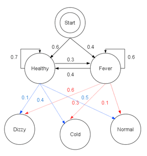
The doctor believes that the health condition of his patients operate as a discrete Markov chain. There are two states, "Healthy" and "Fever", but the doctor cannot observe them directly; they are hidden from him. On each day, there is a certain chance that the patient will tell the doctor he/she is "normal", "cold", or "dizzy", depending on her health condition.
The observations (normal, cold, dizzy) along with a hidden state (healthy, fever) form a hidden Markov model (HMM), and can be represented as follows in the Python programming language:
 1 states = ('Healthy', 'Fever')
 2 observations = ('normal', 'cold', 'dizzy')
 3 start_probability = {'Healthy': 0.6, 'Fever': 0.4}
 4 transition_probability = {
 5    'Healthy' : {'Healthy': 0.7, 'Fever': 0.3},
 6    'Fever' : {'Healthy': 0.4, 'Fever': 0.6}
 7    }
 8 emission_probability = {
 9    'Healthy' : {'normal': 0.5, 'cold': 0.4, 'dizzy': 0.1},
10    'Fever' : {'normal': 0.1, 'cold': 0.3, 'dizzy': 0.6}
11    }
In this piece of code, start_probability represents the doctor's belief about which state the HMM is in when the patient first visits (all he knows is that the patient tends to be healthy). The particular probability distribution used here is not the equilibrium one, which is (given the transition probabilities) approximately {'Healthy': 0.57, 'Fever': 0.43}. The transition_probability represents the change of the health condition in the underlying Markov chain. In this example, there is only a 30% chance that tomorrow the patient will have a fever if he is healthy today. The emission_probability represents how likely the patient is to feel on each day. If he is healthy, there is a 50% chance that he feels normal; if he has a fever, there is a 60% chance that he feels dizzy.
The patient visits three days in a row and the doctor discovers that on the first day she feels normal, on the second day she feels cold, on the third day she feels dizzy. The doctor has a question: what is the most likely sequence of health conditions of the patient that would explain these observations? This is answered by the Viterbi algorithm.
 1 def viterbi(obs, states, start_p, trans_p, emit_p):
 2     V = [{}]
 3     for st in states:
 4         V[0][st] = {"prob": start_p[st] * emit_p[st][obs[0]], "prev": None}
 5     # Run Viterbi when t > 0
 6     for t in range(1, len(obs)):
 7         V.append({})
 8         for st in states:
 9             max_tr_prob = max(V[t-1][prev_st]["prob"]*trans_p[prev_st][st] for prev_st in states)
10             for prev_st in states:
11                 if V[t-1][prev_st]["prob"] * trans_p[prev_st][st] == max_tr_prob:
12                     max_prob = max_tr_prob * emit_p[st][obs[t]]
13                     V[t][st] = {"prob": max_prob, "prev": prev_st}
14                     break
15     for line in dptable(V):
16         print line
17     opt = []
18     # The highest probability
19     max_prob = max(value["prob"] for value in V[-1].values())
20     previous = None
21     # Get most probable state and its backtrack
22     for st, data in V[-1].items():
23         if data["prob"] == max_prob:
24             opt.append(st)
25             previous = st
26             break
27     # Follow the backtrack till the first observation
28     for t in range(len(V) - 2, -1, -1):
29         opt.insert(0, V[t + 1][previous]["prev"])
30         previous = V[t + 1][previous]["prev"]
31
32     print 'The steps of states are ' + ' '.join(opt) + ' with highest probability of %s' % max_prob
33
34 def dptable(V):
35     # Print a table of steps from dictionary
36     yield " ".join(("%12d" % i) for i in range(len(V)))
37     for state in V[0]:
38         yield "%.7s: " % state + " ".join("%.7s" % ("%f" % v[state]["prob"]) for v in V)
The function viterbi takes the following arguments: obs is the sequence of observations, e.g. ['normal', 'cold', 'dizzy']; states is the set of hidden states; start_p is the start probability; trans_p are the transition probabilities; and emit_p are the emission probabilities. For simplicity of code, we assume that the observation sequence obs is non-empty and that trans_p[i][j] and emit_p[i][j] is defined for all states i,j.
In the running example, the forward/Viterbi algorithm is used as follows:
viterbi(observations,
                   states,
                   start_probability,
                   transition_probability,
                   emission_probability)
The output of the script is
1 $ python viterbi_example.py
2          0          1          2
3 Healthy: 0.30000 0.08400 0.00588
4 Fever: 0.04000 0.02700 0.01512
5 The steps of states are Healthy Healthy Fever with highest probability of 0.01512
This reveals that the observations ['normal', 'cold', 'dizzy'] were most likely generated by states ['Healthy', 'Healthy', 'Fever']. In other words, given the observed activities, the patient was most likely to have been healthy both on the first day when she felt normal as well as on the second day when she felt cold, and then she contracted a fever the third day.
The operation of Viterbi's algorithm can be visualized by means of a trellis diagram. The Viterbi path is essentially the shortest path through this trellis. The trellis for the clinic example is shown below; the corresponding Viterbi path is in bold:
See also
- Expectation–maximization algorithm
- Baum–Welch algorithm
- Forward-backward algorithm
- Forward algorithm
- Error-correcting code
- Soft output Viterbi algorithm
- Viterbi decoder
- Hidden Markov model
- Part-of-speech tagging
Notes
- ↑ Xavier Anguera et Al, "Speaker Diarization: A Review of Recent Research", retrieved 19. August 2010, IEEE TASLP
- ↑ 29 Apr 2005, G. David Forney Jr: The Viterbi Algorithm: A Personal History
- 1 2 Daniel Jurafsky; James H. Martin. Speech and Language Processing. Pearson Education International. p. 246.
- ↑ Schmid, Helmut (2004). Efficient parsing of highly ambiguous context-free grammars with bit vectors (PDF). Proc. 20th Int'l Conf. on Computational Linguistics (COLING). doi:10.3115/1220355.1220379.
- ↑ Klein, Dan; Manning, Christopher D. (2003). A* parsing: fast exact Viterbi parse selection (PDF). Proc. 2003 Conf. of the North American Chapter of the Association for Computational Linguistics on Human Language Technology (NAACL). pp. 40–47. doi:10.3115/1073445.1073461.
- ↑ Stanke, M.; Keller, O.; Gunduz, I.; Hayes, A.; Waack, S.; Morgenstern, B. (2006). "AUGUSTUS: Ab initio prediction of alternative transcripts". Nucleic Acids Research. 34: W435. doi:10.1093/nar/gkl200.
- ↑ Qi Wang; Lei Wei; Rodney A. Kennedy (2002). "Iterative Viterbi Decoding, Trellis Shaping,and Multilevel Structure for High-Rate Parity-Concatenated TCM". IEEE Transactions on Communications. 50: 48–55. doi:10.1109/26.975743.
- ↑ A fast maximum-likelihood decoder for convolutional codes (PDF). Vehicular Technology Conference. December 2002. pp. 371–375. doi:10.1109/VETECF.2002.1040367.
- ↑ Xing E, slide 11
References
- Viterbi AJ (April 1967). "Error bounds for convolutional codes and an asymptotically optimum decoding algorithm". IEEE Transactions on Information Theory. 13 (2): 260–269. doi:10.1109/TIT.1967.1054010. (note: the Viterbi decoding algorithm is described in section IV.) Subscription required.
- Feldman J, Abou-Faycal I, Frigo M (2002). "A Fast Maximum-Likelihood Decoder for Convolutional Codes". Vehicular Technology Conference. 1: 371–375. doi:10.1109/VETECF.2002.1040367.
- Forney GD (March 1973). "The Viterbi algorithm". Proceedings of the IEEE. 61 (3): 268–278. doi:10.1109/PROC.1973.9030. Subscription required.
- Press, WH; Teukolsky, SA; Vetterling, WT; Flannery, BP (2007). "Section 16.2. Viterbi Decoding". Numerical Recipes: The Art of Scientific Computing (3rd ed.). New York: Cambridge University Press. ISBN 978-0-521-88068-8.
- Rabiner LR (February 1989). "A tutorial on hidden Markov models and selected applications in speech recognition". Proceedings of the IEEE. 77 (2): 257–286. doi:10.1109/5.18626. (Describes the forward algorithm and Viterbi algorithm for HMMs).
- Shinghal, R. and Godfried T. Toussaint, "Experiments in text recognition with the modified Viterbi algorithm," IEEE Transactions on Pattern Analysis and Machine Intelligence, Vol. PAMI-l, April 1979, pp. 184–193.
- Shinghal, R. and Godfried T. Toussaint, "The sensitivity of the modified Viterbi algorithm to the source statistics," IEEE Transactions on Pattern Analysis and Machine Intelligence, vol. PAMI-2, March 1980, pp. 181–185.
Implementations
- Susa signal processing framework provides the C++ implementation for Forward error correction codes and channel equalization here.
- C#
- Java
- Java 8
- Perl
- Prolog
- Haskell
- Go
- SFIHMM includes code for Viterbi decoding.
External links
- Implementations in Java, F#, Clojure, C# on Wikibooks
- Tutorial on convolutional coding with viterbi decoding, by Chip Fleming
- The history of the Viterbi Algorithm, by David Forney
- A Gentle Introduction to Dynamic Programming and the Viterbi Algorithm
- A tutorial for a Hidden Markov Model toolkit (implemented in C) that contains a description of the Viterbi algorithm