Zernike polynomials

The first 21 Zernike polynomials, ordered vertically by radial degree and horizontally by azimuthal degree

In mathematics, the Zernike polynomials are a sequence of polynomials that are orthogonal on the unit disk. Named after optical physicist Frits Zernike, winner of the 1953 Nobel Prize in Physics and the inventor of phase-contrast microscopy, they play an important role in beam optics.^[1][2]

Definitions

There are even and odd Zernike polynomials. The even ones are defined as

$Z_{n}^{{m}}(\rho ,\varphi )=R_{n}^{m}(\rho )\,\cos(m\,\varphi )\!$

and the odd ones as

$Z_{n}^{{-m}}(\rho ,\varphi )=R_{n}^{m}(\rho )\,\sin(m\,\varphi ),\!$

where m and n are nonnegative integers with n ≥ m, φ is the azimuthal angle, ρ is the radial distance $0\leq \rho \leq 1$, and R^m_n are the radial polynomials defined below. Zernike polynomials have the property of being limited to a range of −1 to +1, i.e. $|Z_{n}^{{m}}(\rho ,\varphi )|\leq 1$. The radial polynomials R^m_n are defined as

$R_{n}^{m}(\rho )=\sum _{{k=0}}^{{{\tfrac {n-m}{2}}}}{\frac {(-1)^{k}\,(n-k)!}{k!\left({\tfrac {n+m}{2}}-k\right)!\left({\tfrac {n-m}{2}}-k\right)!}}\;\rho ^{{n-2\,k}}$

for n − m even, and are identically 0 for n − m odd.

Other representations

Rewriting the ratios of factorials in the radial part as products of binomials shows that the coefficients are integer numbers:

$R_{n}^{m}(\rho )=\sum _{{k=0}}^{{{\tfrac {n-m}{2}}}}(-1)^{k}{\binom {n-k}{k}}{\binom {n-2k}{{\tfrac {n-m}{2}}-k}}\rho ^{{n-2k}}$.

A notation as terminating Gaussian hypergeometric functions is useful to reveal recurrences, to demonstrate that they are special cases of Jacobi polynomials, to write down the differential equations, etc.:

${\displaystyle {\begin{aligned}R_{n}^{m}(\rho )&={\binom {n}{\tfrac {n+m}{2}}}\rho ^{n}\ {}_{2}F_{1}\left(-{\tfrac {n+m}{2}},-{\tfrac {n-m}{2}};-n;\rho ^{-2}\right)\end{aligned}}}$

for n − m even.

Noll's sequential indices

Applications often involve linear algebra, where integrals over products of Zernike polynomials and some other factor build the matrix elements. To enumerate the rows and columns of these matrices by a single index, a conventional mapping of the two indices n and m to a single index j has been introduced by Noll.^[3] The table of this association $Z_{n}^{m}\rightarrow Z_{j}$ starts as follows (sequence A176988 in the OEIS)

n,m | 0,0|1,1| 1,−1 | 2,0| 2,−2 | 2,2|3,−1| 3,1 | 3,−3 | 3,3
j	2| 3 | 4 | 5 | 6 | 7 |8 | 9| 10
n,m |4,0 |4,2 |4,−2|4,4|4,−4|5,1|5,−1|5,3 |5,−3|5,5
j |11 |12 |13 |14|15|16| 17 | 18 |19 |20

The rule is that the even Z (with even azimuthal part m, $\cos(m\varphi )$) obtain even indices j, the odd Z odd indices j. Within a given n, lower values of m obtain lower j.

Properties

Orthogonality

The orthogonality in the radial part reads

$\int _{0}^{1}\rho {\sqrt {2n+2}}R_{n}^{m}(\rho )\,{\sqrt {2n'+2}}R_{{n'}}^{{m}}(\rho )\,d\rho =\delta _{{n,n'}}.$

Orthogonality in the angular part is represented by

$\int _{0}^{{2\pi }}\cos(m\varphi )\cos(m'\varphi )\,d\varphi =\epsilon _{m}\pi \delta _{{|m|,|m'|}},$

$\int _{0}^{{2\pi }}\sin(m\varphi )\sin(m'\varphi )\,d\varphi =(-1)^{{m+m'}}\pi \delta _{{|m|,|m'|}};\quad m\neq 0,$

$\int _{0}^{{2\pi }}\cos(m\varphi )\sin(m'\varphi )\,d\varphi =0,$

where $\epsilon _{m}$ (sometimes called the Neumann factor because it frequently appears in conjunction with Bessel functions) is defined as 2 if $m=0$ and 1 if $m\neq 0$. The product of the angular and radial parts establishes the orthogonality of the Zernike functions with respect to both indices if integrated over the unit disk,

$\int Z_{n}^{m}(\rho ,\varphi )Z_{{n'}}^{{m'}}(\rho ,\varphi )\,d^{2}r={\frac {\epsilon _{m}\pi }{2n+2}}\delta _{{n,n'}}\delta _{{m,m'}},$

where $d^{2}r=\rho \,d\rho \,d\varphi$ is the Jacobian of the circular coordinate system, and where $n-m$ and $n'-m'$ are both even.

A special value is

$R_{n}^{m}(1)=1,\,$

Zernike transform

Any sufficiently smooth real-valued phase field over the unit disk $G(\rho ,\varphi )$ can be represented in terms of its Zernike coefficients (odd and even), just as periodic functions find an orthogonal representation with the Fourier series. We have

$G(\rho ,\varphi )=\sum _{{m,n}}\left[a_{{m,n}}Z_{n}^{{m}}(\rho ,\varphi )+b_{{m,n}}Z_{n}^{{-m}}(\rho ,\varphi )\right],$

where the coefficients can be calculated using inner products. On the space of $L^{2}$ functions on the unit disk, there is an inner product defined by

$\langle F,G\rangle :=\int F(\rho ,\varphi )G(\rho ,\varphi )\rho d\rho d\varphi .$

The Zernike coefficients can then be expressed as follows:

${\begin{aligned}a_{{m,n}}&={\frac {2n+2}{\epsilon _{m}\pi }}\left\langle G(\rho ,\varphi ),Z_{n}^{{m}}(\rho ,\varphi )\right\rangle ,\\b_{{m,n}}&={\frac {2n+2}{\epsilon _{m}\pi }}\left\langle G(\rho ,\varphi ),Z_{n}^{{-m}}(\rho ,\varphi )\right\rangle .\end{aligned}}$

Alternatively, one can use the known values of phase function G on the circular grid to form a system of equations. The phase function is retrieved by the unknown-coefficient weighted product with (known values) of Zernike polynomial across the unit grid. Hence, coefficients can also be found by solving a linear system, for instance by matrix inversion. Fast algorithms to calculate the forward and inverse Zernike transform use symmetry properties of trigonometric functions, separability of radial and azimuthal parts of Zernike polynomials, and their rotational symmetries.

Symmetries

The parity with respect to reflection along the x axis is

$Z_{n}^{{m}}(\rho ,\varphi )=(-1)^{m}Z_{n}^{{m}}(\rho ,-\varphi ).$

The parity with respect to point reflection at the center of coordinates is

$Z_{n}^{m}(\rho ,\varphi )=(-1)^{m}Z_{n}^{m}(\rho ,\varphi +\pi ),$

where $(-1)^{m}$ could as well be written $(-1)^{n}$ because $n-m$ is even for the relevant, non-vanishing values. The radial polynomials are also either even or odd, depending on order n or m:

$R_{n}^{m}(\rho )=(-1)^{n}R_{n}^{m}(-\rho )=(-1)^{m}R_{n}^{m}(-\rho ).$

The periodicity of the trigonometric functions implies invariance if rotated by multiples of $2\pi /m$ radian around the center:

$Z_{n}^{m}\left(\rho ,\varphi +{\tfrac {2\pi k}{m}}\right)=Z_{n}^{m}(\rho ,\varphi ),\qquad k=0,\pm 1,\pm 2,\cdots .$

Recurrence relations

The Zernike polynomials satisfy the following recurrence relation which depends neither on the degree nor on the azimuthal order of the radial polynomials:^[4]

${\displaystyle {\begin{aligned}R_{n}^{m}(\rho )+R_{n-2}^{m}(\rho )=\rho \left[R_{n-1}^{\left|m-1\right|}(\rho )+R_{n-1}^{m+1}(\rho )\right]{\text{ .}}\end{aligned}}}$

From the definition of ${\displaystyle R_{n}^{m}}$ it can be seen that ${\displaystyle R_{m}^{m}(\rho )=\rho ^{m}}$ and ${\displaystyle R_{m+2}^{m}(\rho )=((m+2)\rho ^{2}-(m+1))\rho ^{m}}$. The following three-term recurrence relation^[5] then allows to calculate all other ${\displaystyle R_{n}^{m}(\rho )}$:

${\displaystyle R_{n}^{m}(\rho )={\frac {2(n-1)(2n(n-2)\rho ^{2}-m^{2}-n(n-2))R_{n-2}^{m}(\rho )-n(n+m-2)(n-m-2)R_{n-4}^{m}(\rho )}{(n+m)(n-m)(n-2)}}{\text{ .}}}$

The above relation is especially useful since the derivative of ${\displaystyle R_{n}^{m}}$ can be calculated from two radial Zernike polynomials of adjacent degree:^[5]

${\displaystyle {\frac {\operatorname {d} }{\operatorname {d} \!\rho }}R_{n}^{m}(\rho )={\frac {(2nm(\rho ^{2}-1)+(n-m)(m+n(2\rho ^{2}-1)))R_{n}^{m}(\rho )-(n+m)(n-m)R_{n-2}^{m}(\rho )}{2n\rho (\rho ^{2}-1)}}{\text{ .}}}$

Examples

Radial polynomials

The first few radial polynomials are:

$R_{0}^{0}(\rho )=1\,$

$R_{1}^{1}(\rho )=\rho \,$

$R_{2}^{0}(\rho )=2\rho ^{2}-1\,$

$R_{2}^{2}(\rho )=\rho ^{2}\,$

$R_{3}^{1}(\rho )=3\rho ^{3}-2\rho \,$

$R_{3}^{3}(\rho )=\rho ^{3}\,$

$R_{4}^{0}(\rho )=6\rho ^{4}-6\rho ^{2}+1\,$

$R_{4}^{2}(\rho )=4\rho ^{4}-3\rho ^{2}\,$

$R_{4}^{4}(\rho )=\rho ^{4}\,$

$R_{5}^{1}(\rho )=10\rho ^{5}-12\rho ^{3}+3\rho \,$

$R_{5}^{3}(\rho )=5\rho ^{5}-4\rho ^{3}\,$

$R_{5}^{5}(\rho )=\rho ^{5}\,$

$R_{6}^{0}(\rho )=20\rho ^{6}-30\rho ^{4}+12\rho ^{2}-1\,$

$R_{6}^{2}(\rho )=15\rho ^{6}-20\rho ^{4}+6\rho ^{2}\,$

$R_{6}^{4}(\rho )=6\rho ^{6}-5\rho ^{4}\,$

$R_{6}^{6}(\rho )=\rho ^{6}.\,$

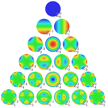
Zernike polynomials

The first few Zernike modes, ordered by Noll index $j$ are^[3] shown below. They are normalized such that

$\int _{0}^{{2\pi }}\int _{0}^{1}Z_{j}^{2}\,\rho \,d\rho \,d\theta =\pi .$

Noll index ($j$)	Radial degree ($n$)	Azimuthal degree ($m$)	$Z_{j}$	Classical name
1	0	0	$1$	Piston
2	1	1	$2\rho \cos \theta$	Tip (lateral position) (X-Tilt)
3	1	−1	$2\rho \sin \theta$	Tilt (lateral position) (Y-Tilt)
4	2	0	${\sqrt {3}}(2\rho ^{2}-1)$	Defocus (longitudinal position)
5	2	−2	${\sqrt {6}}\rho ^{2}\sin 2\theta$	Oblique astigmatism
6	2	2	${\sqrt {6}}\rho ^{2}\cos 2\theta$	Vertical astigmatism
7	3	−1	${\sqrt {8}}(3\rho ^{3}-2\rho )\sin \theta$	Vertical coma
8	3	1	${\sqrt {8}}(3\rho ^{3}-2\rho )\cos \theta$	Horizontal coma
9	3	−3	${\sqrt {8}}\rho ^{3}\sin 3\theta$	Vertical trefoil
10	3	3	${\sqrt {8}}\rho ^{3}\cos 3\theta$	Oblique trefoil
11	4	0	${\sqrt {5}}(6\rho ^{4}-6\rho ^{2}+1)$	Primary spherical
12	4	2	${\sqrt {10}}(4\rho ^{4}-3\rho ^{2})\cos 2\theta$	Vertical secondary astigmatism
13	4	−2	${\sqrt {10}}(4\rho ^{4}-3\rho ^{2})\sin 2\theta$	Oblique secondary astigmatism
14	4	4	${\sqrt {10}}\rho ^{4}\cos 4\theta$	Oblique quadrafoil
15	4	−4	${\sqrt {10}}\rho ^{4}\sin 4\theta$	Vertical quadrafoil

Applications

The functions are a basis defined over the circular support area, typically the pupil planes in classical optical imaging at visible and infrared wavelengths through systems of lenses and mirrors of finite diameter. Their advantages are the simple analytical properties inherited from the simplicity of the radial functions and the factorization in radial and azimuthal functions; this leads, for example, to closed-form expressions of the two-dimensional Fourier transform in terms of Bessel functions. Their disadvantage, in particular if high n are involved, is the unequal distribution of nodal lines over the unit disk, which introduces ringing effects near the perimeter $\rho \approx 1$, which often leads attempts to define other orthogonal functions over the circular disk.

In precision optical manufacturing, Zernike polynomials are used to characterize higher-order errors observed in interferometric analyses, in order to achieve desired system performance.

In optometry and ophthalmology, Zernike polynomials are used to describe aberrations of the cornea or lens from an ideal spherical shape, which result in refraction errors.

They are commonly used in adaptive optics, where they can be used to effectively cancel out atmospheric distortion. Obvious applications for this are IR or visual astronomy and satellite imagery. For example, one of the Zernike terms (for m = 0, n = 2) is called "de-focus". By coupling the output from this term to a control system, an automatic focus can be implemented.

Another application of the Zernike polynomials is found in the Extended Nijboer–Zernike (ENZ) theory of diffraction and aberrations.

Zernike polynomials are widely used as basis functions of image moments. Since Zernike polynomials are orthogonal to each other, Zernike moments can represent properties of an image with no redundancy or overlap of information between the moments. Although Zernike moments are significantly dependent on the scaling and the translation of the object in a region of interest (ROI), their magnitudes are independent of the rotation angle of the object.^[6] Thus, they can be utilized to extract features from images that describe the shape characteristics of an object. For instance, Zernike moments are utilized as shape descriptors to classify benign and malignant breast masses.^[7][8]

Higher dimensions

The concept translates to higher dimensions D if multinomials $x_{1}^{i}x_{2}^{j}\cdots x_{D}^{k}$ in Cartesian coordinates are converted to hyperspherical coordinates, $\rho ^{s},s\leq D$, multiplied by a product of Jacobi polynomials of the angular variables. In $D=3$ dimensions, the angular variables are spherical harmonics, for example. Linear combinations of the powers $\rho ^{s}$ define an orthogonal basis $R_{n}^{{(l)}}(\rho )$ satisfying

$\int _{0}^{1}\rho ^{{D-1}}R_{n}^{{(l)}}(\rho )R_{{n'}}^{{(l)}}(\rho )d\rho =\delta _{{n,n'}}$.

(Note that a factor ${\sqrt {2n+D}}$ is absorbed in the definition of R here, whereas in $D=2$ the normalization is chosen slightly differently. This is largely a matter of taste, depending on whether one wishes to maintain an integer set of coefficients or prefers tighter formulas if the orthogonalization is involved.) The explicit representation is

${\begin{aligned}R_{n}^{{(l)}}(\rho )&={\sqrt {2n+D}}\sum _{{s=0}}^{{{\tfrac {n-l}{2}}}}(-1)^{s}{{\tfrac {n-l}{2}} \choose s}{n-s-1+{\tfrac {D}{2}} \choose {\tfrac {n-l}{2}}}\rho ^{{n-2s}}\\&=(-1)^{{{\tfrac {n-l}{2}}}}{\sqrt {2n+D}}\sum _{{s=0}}^{{{\tfrac {n-l}{2}}}}(-1)^{s}{{\tfrac {n-l}{2}} \choose s}{s-1+{\tfrac {n+l+D}{2}} \choose {\tfrac {n-l}{2}}}\rho ^{{2s+l}}\\&=(-1)^{{{\tfrac {n-l}{2}}}}{\sqrt {2n+D}}{{\tfrac {n+l+D}{2}}-1 \choose {\tfrac {n-l}{2}}}\rho ^{l}\ {}_{2}F_{1}\left(-{\tfrac {n-l}{2}},{\tfrac {n+l+D}{2}};l+{\tfrac {D}{2}};\rho ^{2}\right)\end{aligned}}$

for even $n-l\geq 0$, else identical to zero.

See also

• Jacobi polynomials
• Nijboer–Zernike theory
• Pseudo-Zernike polynomials

References

1. Zernike, F. (1934). "Beugungstheorie des Schneidenverfahrens und Seiner Verbesserten Form, der Phasenkontrastmethode". Physica. 1 (8): 689–704. Bibcode:1934Phy.....1..689Z. doi:10.1016/S0031-8914(34)80259-5.
2. Born, Max, and Wolf, Emil (1999). Principles of Optics: Electromagnetic Theory of Propagation, Interference and Diffraction of Light (7th ed.). Cambridge, UK: Cambridge University Press. p. 986. ISBN 9780521642224.
3. Noll, R. J. (1976). "Zernike polynomials and atmospheric turbulence" (PDF). J. Opt. Soc. Am. 66 (3): 207. Bibcode:1976JOSA...66..207N. doi:10.1364/JOSA.66.000207.
4. Honarvar Shakibaei Asli, Barmak; Raveendran, Paramesran (July 2013). "Recursive formula to compute Zernike radial polynomials" Opt. Lett. (OSA) 38 (14): 2487–2489. doi:10.1364/OL.38.002487
5. Kintner, E. C. (1976). "On the mathematical properties of the Zernike Polynomials". Opt. Acta. 23 (8): 679–680. Bibcode:1976AcOpt..23..679K. doi:10.1080/713819334.
6. Tahmasbi, A. (2010). An Effective Breast Mass Diagnosis System using Zernike Moments. 17th Iranian Conf. on Biomedical Engineering (ICBME'2010). Isfahan, Iran: IEEE. pp. 1–4. doi:10.1109/ICBME.2010.5704941.
7. Tahmasbi, A.; Saki, F.; Shokouhi, S.B. (2011). "Classification of Benign and Malignant Masses Based on Zernike Moments". Computers in Biology and Medicine. 41: 726–735. doi:10.1016/j.compbiomed.2011.06.009.
8. Tahmasbi, A. (2011). A Novel Breast Mass Diagnosis System based on Zernike Moments as Shape and Density Descriptors. 18th Iranian Conf. on Biomedical Engineering (ICBME'2011). Tehran, Iran: IEEE. pp. 100–104. doi:10.1109/ICBME.2011.6168532.

• Weisstein, Eric W. "Zernike Polynomial". MathWorld.

• Callahan, P. G.; De Graef, M. (2012). "Precipitate shape fitting and reconstruction by means of 3D Zernike functions". Model. Simul. Mat. Sci. Engin. 20: 015003. Bibcode:2012MSMSE..20a5003C. doi:10.1088/0965-0393/20/1/015003.
• Campbell, C. E. (2003). "Matrix method to find a new set of Zernike coefficients form an original set when the aperture radius is changed". J. Opt. Soc. Am. A. 20 (2): 209. Bibcode:2003JOSAA..20..209C. doi:10.1364/JOSAA.20.000209.
• Cerjan, C. (2007). "The Zernike-Bessel representation and its application to Hankel transforms". J. Opt. Soc. Am. A. 24 (6): 1609. Bibcode:2007JOSAA..24.1609C. doi:10.1364/JOSAA.24.001609.
• Comastri, S. A.; Perez, L. I.; Perez, G. D.; Martin, G.; Bastida Cerjan, K. (2007). "Zernike expansion coefficients: rescaling and decentering for different pupils and evaluation of corneal aberrations". J. Opt. Soc. Am. A. 9 (3): 209–221. Bibcode:2007JOptA...9..209C. doi:10.1088/1464-4258/9/3/001.
• Conforti, G. (1983). "Zernike aberration coefficients from Seidel and higher-order power-series coefficients". Opt. Lett. 8 (7): 407–408. Bibcode:1983OptL....8..407C. doi:10.1364/OL.8.000407.
• Dai, G-m.; Mahajan, V. N. (2007). "Zernike annular polynomials and atmospheric turbulence". J. Opt. Soc. Am. A. 24: 139. Bibcode:2007JOSAA..24..139D. doi:10.1364/JOSAA.24.000139.
• Dai, G-m. (2006). "Scaling Zernike expansion coefficients to smaller pupil sizes: a simpler formula". J. Opt. Soc. Am. A. 23 (3): 539. Bibcode:2006JOSAA..23..539D. doi:10.1364/JOSAA.23.000539.
• Díaz, J. A.; Fernández-Dorado, J.; Pizarro, C.; Arasa, J. (2009). "Zernike Coefficients for Concentric, Circular, Scaled Pupils: An Equivalent Expression". Journal of Modern Optics. 56 (1): 149–155. Bibcode:2009JMOp...56..149D. doi:10.1080/09500340802531224.
• Díaz, J. A.; Fernández-Dorado, J. "Zernike Coefficients for Concentric, Circular, Scaled Pupils". from The Wolfram Demonstrations Project.
• Farokhi, Sajad; Shamsuddin, Siti Mariyam; Flusser, Jan; Sheikh, U.U; Khansari, Mohammad; Jafari-Khouzani, Kourosh (2013). "Rotation and noise invariant near-infrared face recognition by means of Zernike moments and spectral regression discriminant analysis". Journal of Electronic Imaging. 22 (1): 013030. Bibcode:2013JEI....22a3030F. doi:10.1117/1.JEI.22.1.013030.
• Gu, J.; Shu, H. Z.; Toumoulin, C.; Luo, L. M. (2002). "A novel algorithm for fast computation of Zernike moments". Pattern Recogn. 35 (12): 2905–2911. doi:10.1016/S0031-3203(01)00194-7.
• Herrmann, J. (1981). "Cross coupling and aliasing in modal wave-front estimation". J. Opt. Soc. Am. 71 (8): 989. Bibcode:1981JOSA...71..989H. doi:10.1364/JOSA.71.000989.
• Hu, P. H.; Stone, J.; Stanley, T. (1989). "Application of Zernike polynomials to atmospheric propagation problems". J. Opt. Soc. Am. A. 6 (10): 1595. Bibcode:1989JOSAA...6.1595H. doi:10.1364/JOSAA.6.001595.
• Kintner, E. C. (1976). "On the mathematical properties of the Zernike Polynomials". Opt. Acta. 23 (8): 679–680. Bibcode:1976AcOpt..23..679K. doi:10.1080/713819334.
• Lawrence, G. N.; Chow, W. W. (1984). "Wave-front tomography by Zernike Polynomial decomposition". Opt. Lett. 9 (7): 267. Bibcode:1984OptL....9..267L. doi:10.1364/OL.9.000267.
• Liu, Haiguang; Morris, Richard J.; Hexemer, A.; Grandison, Scott; Zwart, Peter H. (2012). "Computation of small-angle scattering profiles with three-dimensional Zernike polynomials". Acta Crystallogr. A. 68 (2): 278–285. doi:10.1107/S010876731104788X.
• Lundström, L.; Unsbo, P. (2007). "Transformation of Zernike coefficients: scaled, translated and rotated wavefronts with circular and elliptical pupils". J. Opt. Soc. Am. A. 24 (3): 569. Bibcode:2007JOSAA..24..569L. doi:10.1364/JOSAA.24.000569.
• Mahajan, V. N. (1981). "Zernike annular polynomials for imaging systems with annular pupils". J. Opt. Soc. Am. 71: 75. Bibcode:1981JOSA...71...75M. doi:10.1364/JOSA.71.000075.
• Mathar, R. J. (2007). "Third Order Newton's Method for Zernike Polynomial Zeros". arXiv:0705.1329 [math.NA].
• Mathar, R. J. (2009). "Zernike Basis to Cartesian Transformations". Serbian Astronomical Journal. 179 (179): 107–120. arXiv:0809.2368. Bibcode:2009SerAj.179..107M. doi:10.2298/SAJ0979107M.
• Prata Jr, A.; Rusch, W. V. T. (1989). "Algorithm for computation of Zernike polynomials expansion coefficients". Appl. Opt. 28 (4): 749. Bibcode:1989ApOpt..28..749P. doi:10.1364/AO.28.000749.
• Schwiegerling, J. (2002). "Scaling Zernike expansion coefficients to different pupil sizes". J. Opt. Soc. Am. A. 19 (10): 1937. Bibcode:2002JOSAA..19.1937S. doi:10.1364/JOSAA.19.001937.
• Sheppard, C. J. R.; Campbell, S.; Hirschhorn, M. D. (2004). "Zernike expansion of separable functions in Cartesian coordinates". Appl. Opt. 43 (20): 3963. Bibcode:2004ApOpt..43.3963S. doi:10.1364/AO.43.003963.
• Shu, H.; Luo, L.; Han, G.; Coatrieux, J.-L. (2006). "General method to derive the relationship between two sets of Zernike coefficients corresponding to different aperture sizes". J. Opt. Soc. Am. A. 23 (8): 1960. Bibcode:2006JOSAA..23.1960S. doi:10.1364/JOSAA.23.001960.
• Swantner, W.; Chow, W. W. (1994). "Gram-Schmidt orthogonalization of Zernike polynomials for general aperture shapes". Appl. Opt. 33 (10): 1832. Bibcode:1994ApOpt..33.1832S. doi:10.1364/AO.33.001832.
• Tango, W. J. (1977). "The circle polynomials of Zernike and their application in optics". Appl. Phys. A. 13 (4): 327–332. Bibcode:1977ApPhy..13..327T. doi:10.1007/BF00882606.
• Tyson, R. K. (1982). "Conversion of Zernike aberration coefficients to Seidel and higher-order power series aberration coefficients". Opt. Lett. 7 (6): 262. Bibcode:1982OptL....7..262T. doi:10.1364/OL.7.000262.
• Wang, J. Y.; Silva, D. E. (1980). "Wave-front interpretation with Zernike Polynomials". Appl. Opt. 19 (9): 1510. Bibcode:1980ApOpt..19.1510W. doi:10.1364/AO.19.001510.
• Barakat, R. (1980). "Optimum balanced wave-front aberrations for radially symmetric amplitude distributions: Generalizations of Zernike polynomials". J. Opt. Soc. Am. 70 (6): 739. Bibcode:1980JOSA...70..739B. doi:10.1364/JOSA.70.000739.
• Bhatia, A. B.; Wolf, E. (1952). "The Zernike circle polynomials occurring in diffraction theory". Proc. Phys. Soc. B. 65 (11): 909–910. Bibcode:1952PPSB...65..909B. doi:10.1088/0370-1301/65/11/112.
• ten Brummelaar, T. A. (1996). "Modeling atmospheric wave aberrations and astronomical instrumentation using the polynomials of Zernike". Opt. Commun. 132 (3–4): 329–342. Bibcode:1996OptCo.132..329T. doi:10.1016/0030-4018(96)00407-5.
• Novotni, M.; Klein, R. "3D Zernike Descriptors for Content Based Shape Retrieval" (PDF). Proceedings of the 8th ACM Symposium on Solid Modeling and Applications.
• Novotni, M.; Klein, R. (2004). "Shape retrieval using 3D Zernike descriptors" (PDF). Computer Aided Design. 36 (11): 1047–1062. doi:10.1016/j.cad.2004.01.005.
• Farokhi, Sajad; Shamsuddin, Siti Mariyam; Sheikh, U.U; Flusser, Jan (2014). "Near Infrared Face Recognition: A Comparison of Moment-Based Approaches" (PDF). Lecture Notes in Electrical Engineering. Springer. 291 (1): 129–135. doi:10.1007/978-981-4585-42-2_15.
• Farokhi, Sajad; Shamsuddin, Siti Mariyam; Flusser, Jan; Sheikh, U.U; Khansari, Mohammad; Jafari-Khouzani, Kourosh (2014). "Near infrared face recognition by combining Zernike moments and undecimated discrete wavelet transform". Digital Signal Processing. 31 (1): 13–27. doi:10.1016/j.dsp.2014.04.008.

External links

• The Extended Nijboer-Zernike website
• MATLAB code for fast calculation of Zernike moments
• Python/NumPy library for calculating Zernike polynomials
• Zernike aberrations at Telescope Optics
• Example: using WolframAlpha to plot Zernike Polynomials