Algebraic curve
In mathematics, a plane real algebraic curve is the set of points on the Euclidean plane whose coordinates are zeros of some polynomial in two variables. More generally an algebraic curve is similar but may be embedded in a higher dimensional space or defined over some more general field.
For example, the unit circle is a real algebraic curve, being the set of zeros of the polynomial x2 + y2 – 1.
Various technical considerations result in the complex zeros of a polynomial being considered as belonging to the curve. Also, the notion of algebraic curve has been generalized to allow the coefficients of the defining polynomial and the coordinates of the points of the curve to belong to any field, leading to the following definition.
In algebraic geometry, a plane affine algebraic curve defined over a field k is the set of points of K2 whose coordinates are zeros of some bivariate polynomial with coefficients in k, where K is some algebraically closed extension of k. The points of the curve with coordinates in k are the k-points of the curve and, all together, are the k part of the curve.
For example, (2,√−3) is a point of the curve defined by x2 + y2 − 1 = 0 and the usual unit circle is the real part of this curve. The term "unit circle" may refer to all the complex points as well as to only the real points, the exact meaning usually clear from the context. The equation x2 + y2 + 1 = 0 defines an algebraic curve, whose real part is empty.
More generally, one may consider algebraic curves that are not contained in the plane, but in a space of higher dimension. A curve that is not contained in some plane is called a skew curve. The simplest example of a skew algebraic curve is the twisted cubic. One may also consider algebraic curves contained in the projective space and even algebraic curves that are defined independently to any embedding in an affine or projective space. This leads to the most general definition of an algebraic curve:
In algebraic geometry, an algebraic curve is an algebraic variety of dimension one.
In Euclidean geometry
An algebraic curve in the Euclidean plane is the set of the points whose coordinates are the solutions of a bivariate polynomial equation p(x, y) = 0. This equation is often called the implicit equation of the curve, by opposition to the curves that are the graph of a function defining explicitly y as a function of x.
Given a curve given by such an implicit equation, the first problems that occur is to determine the shape of the curve and to draw it. These problems are not as easy to solve as in the case of the graph of a function, for which y may easily be computed for various values of x. The fact that the defining equation is a polynomial implies that the curve has some structural properties that may help to solve these problems.
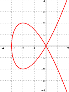
Every algebraic curve may be uniquely decomposed into a finite number of smooth monotone arcs (also called branches) connected by some points sometimes called "remarkable points". A smooth monotone arc is the graph of a smooth function which is defined and monotone on an open interval of the x-axis. In each direction, an arc is either unbounded (usually called an infinite arc) or has an end point which is either a singular point (this will be defined below) or a point with a tangent parallel to one of the coordinate axes.
For example, for the Tschirnhausen cubic of the figure, there are two infinite arcs having the origin (0,0) as end point. This point is the only singular point of the curve. There are two arcs having this singular point as one end point and having a second end point with a horizontal tangent. Finally, there are two other arcs having these points with horizontal tangent as first end point and sharing the unique point with vertical tangent as second end point. On the other hand, the sinusoid is certainly not an algebraic curve, having an infinite number of monotone arcs.
To draw an algebraic curve, it is important to know the remarkable points and their tangents, the infinite branches and their asymptote (if any) and the way in which the arcs connect them. It is also useful to consider also the inflection points as remarkable points. When all this information is drawn on a paper sheet, the shape of the curve appears usually rather clearly. If not it suffices to add a few other points and their tangents to get a good description of the curve.
The methods for computing the remarkable points and their tangents are described below, after section Projective curves.
Plane projective curves
It is often desirable to consider curves in the projective space. An algebraic curve in the projective plane or plane projective curve is the set of the points in a projective plane whose projective coordinates are zeros of a homogeneous polynomial in three variables P(x, y, z).
Every affine algebraic curve of equation p(x, y) = 0 may be completed into the projective curve of equation where


is the result of the homogenization of p. Conversely, if P(x, y, z) = 0 is the homogeneous equation of a projective curve, then P(x, y, 1) = 0 is the equation of an affine curve, which consists of the points of the projective curve whose third projective coordinate is not zero. These two operations are reciprocal one to the other, as and, if p is defined by , then , as soon as the homogeneous polynomial P is not divisible by z.


For example, the projective curve of equation x2 + y2 − z2 is the projective completion of the unit circle of equation x2 + y2 − 1 = 0.
This allows to consider that an affine curve and its projective completion are the same curve, or, more precisely that the affine curve is a part of the projective curve that is large enough to well define the "complete" curve. This point of view is commonly expressed by calling "points at infinity" of the affine curve the points (in finite number) of the projective completion that do not belong to the affine part.
Projective curves are frequently studied for themselves. They are also useful for the study of affine curves. For example, if p(x, y) is the polynomial defining an affine curve, beside the partial derivatives and , it is useful to consider the derivative at infinity


For example, the equation of the tangent of the affine curve of equation p(x, y) = 0 at a point (a, b) is

Remarkable points of a plane curve
In this section, we consider a plane algebraic curve defined by a bivariate polynomial p(x, y) and its projective completion, defined by the homogenization of p.

Intersection with a line
Knowing the points of intersection of a curve with a given line is frequently useful. The intersection with the axes of coordinates and the asymptotes are useful to draw the curve. Intersecting with a line parallel to the axes allows one to find at least a point in each branch of the curve. If an efficient root-finding algorithm is available, this allows to draw the curve by plotting the intersection point with all the lines parallel to the y-axis and passing through each pixel on the x-axis.
If the polynomial defining the curve has degree d, any line cuts the curve in at most d points. Bézout's theorem asserts that this number is exactly d, if the points are searched in the projective plane over an algebraically closed field (for example the complex numbers), and counted with their multiplicity. The method of computation that follows proves again this theorem, in this simple case.
To compute the intersection of the curve defined by the polynomial p with the line of equation ax+by+c = 0, one solves in x (or in y if a = 0) the equation of the line. Substituting the result in p, one gets a univariate equation q(y) = 0 (or q(x) = 0, if the equation of the line has been solved in y), whose roots are one coordinate of the intersection points. The other coordinate is deduced from the equation of the line. The multiplicity of an intersection point is the multiplicity of the corresponding root. There is an intersection point at infinity, if the degree of q is lower than the degree of p; the multiplicity of such an intersection point at infinity is the difference of the degrees of p and q.
Tangent at a point
The tangent at a point (a, b) of the curve is the line of equation , like for every differentiable curve defined by an implicit equation. In the case of polynomials, another formula for the tangent has a simpler constant term and is more symmetric:


where is the derivative at infinity. The equivalence of the two equations results from Euler's homogeneous function theorem applied to P.

If the tangent is not defined and the point is a singular point.

This extends immediately to the projective case: The equation of the tangent of at the point of projective coordinates (a:b:c) of the projective curve of equation P(x, y, z) = 0 is

and the points of the curves that are singular are the points such that

(The condition P(a, b, c) = 0 is implied by these conditions, by Euler's homogeneous function theorem.)
Asymptotes
Every infinite branch of an algebraic curve corresponds to a point at infinity on the curve, that is a point of the projective completion of the curve that does not belongs to its affine part. The corresponding asymptote is the tangent of the curve at that point. The general formula for a tangent to a projective curve may apply, but it is worth to make it explicit in this case.
Let be the decomposition of the polynomial defining the curve into its homogeneous parts, where pi is the sum of the monomials of p of degree i. It follows that


and

A point at infinity of the curve is a zero of p of the form (a, b, 0). Equivalently, (a, b) is a zero of pd. The fundamental theorem of algebra implies that, over an algebraically closed field (typically, the field of complex numbers), pd factors into a product of linear factors. Each factor defines a point at infinity on the curve: if bx − ay is such a factor, then it defines the point at infinity (a, b, 0). Over the reals, pd factors into linear and quadratic factors. The irreducible quadratic factors define non-real points at infinity, and the real points are given by the linear factors. If (a, b, 0) is a point at infinity of the curve, one says that (a, b) is an asymptotic direction. Setting q = pd the equation of the corresponding asymptote is

If and the asymptote is the line at infinity, and, in the real case, the curve has a branch that looks like a parabola. In this case one says that the curve has a parabolic branch. If


the curve has a singular point at infinity and may have several asymptotes. They may be computed by the method of computing the tangent cone of a singular point.
Singular points
The singular points of a curve of degree d defined by a polynomial p(x,y) of degree d are the solutions of the system of equations:

In characteristic zero, this system is equivalent with

where, with the notation of the preceding section, The systems are equivalent because of Euler's homogeneous function theorem. The latter system has the advantage of having its third polynomial of degree d-1 instead of d.

Similarly, for a projective curve defined by a homogeneous polynomial P(x,y,z) of degree d, the singular points have the solutions of the system

as homogeneous coordinates. (In positive characteristic, the equation has to be added to the system.)

This implies that the number of singular points is finite as long as p(x,y) or P(x,y,z) is square free. Bézout's theorem implies thus that the number of singular points is at most (d−1)2, but this bound is not sharp because the system of equations is overdetermined. If reducible polynomials are allowed, the sharp bound is d(d−1)/2, this value being reached when the polynomial factors in linear factors, that is if the curve is the union of d lines. For irreducible curves and polynomials, the number of singular points is at most (d−1)(d−2)/2, because of the formula expressing the genus in term of the singularities (see below). The maximum is reached by the curves of genus zero whose all singularities have multiplicity two and distinct tangents (see below).
The equation of the tangents at a singular point is given by the nonzero homogeneous part of lowest degree in the Taylor series of the polynomial at the singular point. When one changes the coordinates to put the singular point at the origin, the equation of the tangents at the singular point is thus the nonzero homogeneous part of lowest degree of the polynomial, and the multiplicity of the singular point is the degree of this homogeneous part.
Non-plane algebraic curves
An algebraic curve is an algebraic variety of dimension one. This implies that an affine curve in an affine space of dimension n is defined by, at least, n−1 polynomials in n variables. To define a curve, these polynomials must generate a prime ideal of Krull dimension 1. This condition is not easy to test in practice. Therefore the following way to represent non-plane curves may be preferred.
Let be n − 1 polynomials in two variables x1 and x2 such that f is irreducible. The points in the affine space of dimension n such whose coordinates satisfy the equations and inequations


are all the points of an algebraic curve in which a finite number of points have been removed. This curve is defined by a system of generators of the ideal of the polynomials h such that it exists an integer k such belongs to the ideal generated by . This representation is a rational equivalence between the curve and the plane curve defined by f. Every algebraic curve may be represented in this way. However, a linear change of variables may be needed in order to make almost always injective the projection on the two first variables. When a change of variables is needed, almost every change is convenient, as soon as it is defined over an infinite field.


This representation allows us to deduce easily any property of a non-plane algebraic curve, including its graphical representation, from the corresponding property of its plane projection.
For a curve defined by its implicit equations, above representation of the curve may easily deduced from a Gröbner basis for a block ordering such that the block of the smaller variables is (x1, x2). The polynomial f is the unique polynomial in the base that depends only of x1 and x2. The fractions gi/g0 are obtained by choosing, for i = 3, ..., n, a polynomial in the basis that is linear in xi and depends only on x1, x2 and xi. If these choices are not possible, this means either that the equations define an algebraic set that is not a variety, or that the variety is not of dimension one, or that one must change of coordinates. The latter case occurs when f exists and is unique, and, for i = 3, ..., n, there exist polynomials whose leading monomial depends only on x1, x2 and xi.
Algebraic function fields
The study of algebraic curves can be reduced to the study of irreducible algebraic curves: those curves that cannot be written as the union of two smaller curves. Up to birational equivalence, the irreducible curves over a field F are categorically equivalent to algebraic function fields in one variable over F. Such an algebraic function field is a field extension K of F that contains an element x which is transcendental over F, and such that K is a finite algebraic extension of F(x), which is the field of rational functions in the indeterminate x over F.
For example, consider the field C of complex numbers, over which we may define the field C(x) of rational functions in C. If y2 = x3 − x − 1, then the field C(x, y) is an elliptic function field. The element x is not uniquely determined; the field can also be regarded, for instance, as an extension of C(y). The algebraic curve corresponding to the function field is simply the set of points (x, y) in C2 satisfying y2 = x3 − x − 1.
If the field F is not algebraically closed, the point of view of function fields is a little more general than that of considering the locus of points, since we include, for instance, "curves" with no points on them. For example, if the base field F is the field R of real numbers, then x2 + y2 = −1 defines an algebraic extension field of R(x), but the corresponding curve considered as a subset of R2 has no points. The equation x2 + y2 = −1 does define an irreducible algebraic curve over R in the scheme sense (an integral, separated one-dimensional schemes of finite type over R). In this sense, the one-to-one correspondence between irreducible algebraic curves over F (up to birational equivalence) and algebraic function fields in one variable over F holds in general.
Two curves can be birationally equivalent (i.e. have isomorphic function fields) without being isomorphic as curves. The situation becomes easier when dealing with nonsingular curves, i.e. those that lack any singularities. Two nonsingular projective curves over a field are isomorphic if and only if their function fields are isomorphic.
Tsen's theorem is about the function field of an algebraic curve over an algebraically closed field.
Complex curves and real surfaces
A complex projective algebraic curve resides in n-dimensional complex projective space CPn. This has complex dimension n, but topological dimension, as a real manifold, 2n, and is compact, connected, and orientable. An algebraic curve over C likewise has topological dimension two; in other words, it is a surface.
The topological genus of this surface, that is the number of handles or donut holes, is equal to the geometric genus of the algebraic curve that may be computed by algebraic means. In short, if one consider a plane projection of a nonsingular curve that has degree d and only ordinary singularities (singularities of multiplicity two with distinct tangents), then the genus is (d − 1)(d − 2)/2 − k, where k is the number of these singularities.
Compact Riemann surfaces
A Riemann surface is a connected complex analytic manifold of one complex dimension, which makes it a connected real manifold of two dimensions. It is compact if it is compact as a topological space.
There is a triple equivalence of categories between the category of smooth irreducible projective algebraic curves over C (with non-constant regular maps as morphisms), the category of compact Riemann surfaces (with non-constant holomorphic maps as morphisms), and the opposite of the category of algebraic function fields in one variable over C (with field homomorphisms that fix C as morphisms). This means that in studying these three subjects we are in a sense studying one and the same thing. It allows complex analytic methods to be used in algebraic geometry, and algebraic-geometric methods in complex analysis, and field-theoretic methods to be used in both. This is characteristic of a much wider class of problems in algebraic geometry.
See also algebraic geometry and analytic geometry for more general theory.
Singularities
Using the intrinsic concept of tangent space, points P on an algebraic curve C are classified as smooth (synonymous: non-singular), or else singular. Given n−1 homogeneous polynomials in n+1 variables, we may find the Jacobian matrix as the (n−1)×(n+1) matrix of the partial derivatives. If the rank of this matrix is n−1, then the polynomials define an algebraic curve (otherwise they define an algebraic variety of higher dimension). If the rank remains n−1 when the Jacobian matrix is evaluated at a point P on the curve, then the point is a smooth or regular point; otherwise it is a singular point. In particular, if the curve is a plane projective algebraic curve, defined by a single homogeneous polynomial equation f(x,y,z) = 0, then the singular points are precisely the points P where the rank of the 1×(n+1) matrix is zero, that is, where

Since f is a polynomial, this definition is purely algebraic and makes no assumption about the nature of the field F, which in particular need not be the real or complex numbers. It should of course be recalled that (0,0,0) is not a point of the curve and hence not a singular point.
Similarly, for an affine algebraic curve defined by a single polynomial equation f(x,y) = 0, then the singular points are precisely the points P of the curve where the rank of the 1×n Jacobian matrix is zero, that is, where

The singularities of a curve are not birational invariants. However, locating and classifying the singularities of a curve is one way of computing the genus, which is a birational invariant. For this to work, we should consider the curve projectively and require F to be algebraically closed, so that all the singularities which belong to the curve are considered.
Classification of singularities
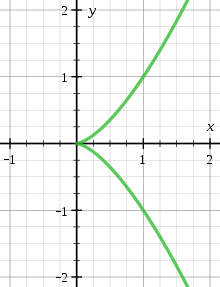
Singular points include multiple points where the curve crosses over itself, and also various types of cusp, for example that shown by the curve with equation x3 = y2 at (0,0).
A curve C has at most a finite number of singular points. If it has none, it can be called smooth or non-singular. Commonly, this definition is understood over an algebraically closed field and for a curve C in projective space (i.e., complete in the sense of algebraic geometry). For example, the curve of equation is considered as singular, as having a singular point (a cusp) at infinity.

The singular points are classified by means of several invariants. The multiplicity m is defined as the maximum integer such that the derivatives of f to all orders up to m – 1 vanish (also the minimal intersection number between the curve and a straight line at P). Intuitively, a singular point has delta invariant δ if it concentrates δ ordinary double points at P. To make this precise, the blow up process produces so-called infinitely near points, and summing m(m−1)/2 over the infinitely near points, where m is their multiplicity, produces δ. For an irreducible and reduced curve and a point P we can define δ algebraically as the length of where is the local ring at P and is its integral closure.[1]


The Milnor number μ of a singularity is the degree of the mapping grad f(x,y)/|grad f(x,y)| on the small sphere of radius ε, in the sense of the topological degree of a continuous mapping, where grad f is the (complex) gradient vector field of f. It is related to δ and r by the Milnor-Jung formula,
- μ = 2δ − r + 1.
Here, the branching number r of P is the number of locally irreducible branches at P. For example, r = 1 at an ordinary cusp, and r = 2 at an ordinary double point. Note that m is at least r, and that P is singular if and only if m is at least 2. Moreover, δ is at least m(m-1)/2.
Computing the delta invariants of all of the singularities allows the genus g of the curve to be determined; if d is the degree, then

where the sum is taken over all singular points P of the complex projective plane curve. It is called the genus formula.
Assign the invariants [m, δ, r] to a singularity, where m is the multiplicity, δ is the delta-invariant, and r is the branching number. Then an ordinary cusp is a point with invariants [2,1,1] and an ordinary double point is a point with invariants [2,1,2], and an ordinary m-multiple point is a point with invariants [m, m(m−1)/2, m].
Examples of curves
Rational curves
A rational curve, also called a unicursal curve, is any curve which is birationally equivalent to a line, which we may take to be a projective line; accordingly, we may identify the function field of the curve with the field of rational functions in one indeterminate F(x). If F is algebraically closed, this is equivalent to a curve of genus zero; however, the field of all real algebraic functions defined on the real algebraic variety x2+y2 = −1 is a field of genus zero which is not a rational function field.
Concretely, a rational curve of dimension n over F can be parameterized (except for isolated exceptional points) by means of n rational functions defined in terms of a single parameter t; by clearing denominators we can turn this into n+1 polynomial functions in projective space. An example would be the rational normal curve.
Any conic section defined over F with a rational point in F is a rational curve. It can be parameterized by drawing a line with slope t through the rational point, and intersection with the plane quadratic curve; this gives a polynomial with F-rational coefficients and one F-rational root, hence the other root is F-rational (i.e., belongs to F) also.
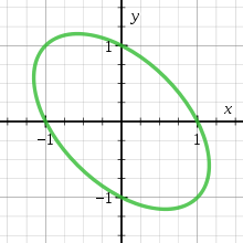
For example, consider the ellipse x2 + xy + y2 = 1, where (−1, 0) is a rational point. Drawing a line with slope t from (−1,0), y = t(x+1), substituting it in the equation of the ellipse, factoring, and solving for x, we obtain

We then have that the equation for y is

which defines a rational parameterization of the ellipse and hence shows the ellipse is a rational curve. All points of the ellipse are given, except for (−1,1), which corresponds to t = ∞; the entire curve is parameterized therefore by the real projective line.
Such a rational parameterization may be considered in the projective space by equating the first projective coordinates to the numerators of the parameterization and the last one to the common denominator. As the parameter is defined in a projective line, the polynomials in the parameter should be homogenized. For example, the projective parameterization of above ellipse is

Eliminating T and U between these equations we get again the projective equation of the ellipse

which may be easily obtained directly by homogenizing above equation.
Many of the curves on Wikipedia's list of curves are rational, and hence have similar rational parameterizations.
Elliptic curves
An elliptic curve may be defined as any curve of genus one with a rational point: a common model is a nonsingular cubic curve, which suffices to model any genus one curve. In this model the distinguished point is commonly taken to be an inflection point at infinity; this amounts to requiring that the curve can be written in Tate-Weierstrass form, which in its projective version is

Elliptic curves carry the structure of an abelian group with the distinguished point as the identity of the group law. In a plane cubic model three points sum to zero in the group if and only if they are collinear. For an elliptic curve defined over the complex numbers the group is isomorphic to the additive group of the complex plane modulo the period lattice of the corresponding elliptic functions.
The intersection of two quadric surfaces is in general a nonsingular curve of genus one and degree four, and thus an elliptic curve, if it has a rational point. In special cases, the intersection either may be a rational singular quartic, or is decomposed in curves of smaller degrees which are not always distinct (either a cubic curve and a line, or two conics, or a conic and two lines, or four lines).
Curves of genus greater than one
Curves of genus greater than one differ markedly from both rational and elliptic curves. Such curves defined over the rational numbers, by Faltings' theorem, can have only a finite number of rational points, and they may be viewed as having a hyperbolic geometry structure. Examples are the hyperelliptic curves, the Klein quartic curve, and the Fermat curve xn + yn = zn when n is greater than three.
See also
Classical algebraic geometry
Modern algebraic geometry
Geometry of Riemann surfaces
References
| Wikimedia Commons has media related to Algebraic curves. |
- Egbert Brieskorn and Horst Knörrer, Plane Algebraic Curves, John Stillwell, translator, Birkhäuser, 1986
- Claude Chevalley, Introduction to the Theory of Algebraic Functions of One Variable, American Mathematical Society, Mathematical Surveys Number VI, 1951
- Hershel M. Farkas and Irwin Kra, Riemann Surfaces, Springer, 1980
- W. Fulton, Algebraic Curves: an introduction to algebraic geometry.
- C.G. Gibson, Elementary Geometry of Algebraic Curves: An Undergraduate Introduction, Cambridge University Press, 1998.
- Phillip A. Griffiths, Introduction to Algebraic Curves, Kuniko Weltin, trans., American Mathematical Society, Translation of Mathematical Monographs volume 70, 1985 revision
- Robin Hartshorne, Algebraic Geometry, Springer, 1977
- Shigeru Iitaka, Algebraic Geometry: An Introduction to the Birational Geometry of Algebraic Varieties, Springer, 1982
- John Milnor, Singular Points of Complex Hypersurfaces, Princeton University Press, 1968
- George Salmon, Higher Plane Curves, Third Edition, G. E. Stechert & Co., 1934
- Jean-Pierre Serre, Algebraic Groups and Class Fields, Springer, 1988
- Ernst Kötter (1887). "Grundzüge einer rein geometrischen Theorie der algebraischen ebenen Kurven (Fundamentals of a purely geometrical theory of algebraic plane curves)". Transactions of the Royal Academy of Berlin. — gained the 1886 Academy prize[2]
Notes
- ↑ Hartshorne, Algebraic Geometry, IV Ex. 1.8.
- ↑ Norman Fraser (Feb 1888). "Kötter's synthetic geometry of algebraic curves". Proceedings of the Edinburgh Mathematical Society. 7: 46–61. Here: p.46
| Curves |  | |
|---|---|---|
| Helices | ||
| Spirals | ||