Autonomous system (mathematics)
| Differential equations | |||||
|---|---|---|---|---|---|
 Navier–Stokes differential equations used to simulate airflow around an obstruction. | |||||
| Classification | |||||
|
Types
|
|||||
|
Relation to processes |
|||||
| Solution | |||||
|
General topics |
|||||
In mathematics, an autonomous system or autonomous differential equation is a system of ordinary differential equations which does not explicitly depend on the independent variable. When the variable is time, they are also called time-invariant systems.
Many laws in physics, where the independent variable is usually assumed to be time, are expressed as autonomous systems because it is assumed the laws of nature which hold now are identical to those for any point in the past or future.
Autonomous systems are closely related to dynamical systems. Any autonomous system can be transformed into a dynamical system and, using very weak assumptions, a dynamical system can be transformed into an autonomous system.
Definition
An autonomous system is a system of ordinary differential equations of the form

where x takes values in n-dimensional Euclidean space and t is usually time.
It is distinguished from systems of differential equations of the form

in which the law governing the rate of motion of a particle depends not only on the particle's location, but also on time; such systems are not autonomous.
Properties
Let be a unique solution of the initial value problem for an autonomous system

- .

Then solves

- .

Indeed, denoting we have and , thus


- .

For the initial condition, the verification is trivial,
- .

Example
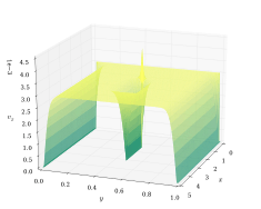
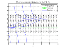
The equation is autonomous, since the independent variable, let us call it , does not explicitly appear in the equation. To plot the slope field and isocline for this equation, one can use the following code in GNU Octave/MATLAB


Ffun = @(X,Y)(2-Y).*Y;           % function f(x,y)=(2-y)y
[X,Y]=meshgrid(0:.2:6,-1:.2:3);  % choose the plot sizes
DY=Ffun(X,Y); DX=ones(size(DY)); % generate the plot values
quiver(X,Y,DX,DY, 'k');          % plot the direction field in black
hold on;
contour(X,Y,DY,[0 1 2], 'g');    % add the isoclines(0 1 2) in green
title('Slope field and isoclines for f(x,y)=(2-y)y')
One can observe from the plot that the function is -invariant, and so is the shape of the solution, i.e. for any shift .


Solving the equation symbolically in MATLAB, by running
y=dsolve('Dy=(2-y)*y','x'); % solve the equation symbolically
we obtain two equilibrium solutions, and , and a third solution involving an unknown constant ,


y(3)=-2/(exp(C3 - 2*x) - 1)
Picking up some specific values for the initial condition, we can add the plot of several solutions
y1=dsolve('Dy=(2-y)*y','y(1)=1','x'); % solve the initial value problem symbolically
y2=dsolve('Dy=(2-y)*y','y(2)=1','x'); % for different initial conditions
y3=dsolve('Dy=(2-y)*y','y(3)=1','x'); y4=dsolve('Dy=(2-y)*y','y(1)=3','x');
y5=dsolve('Dy=(2-y)*y','y(2)=3','x'); y6=dsolve('Dy=(2-y)*y','y(3)=3','x');
ezplot(y1, [0 6]); ezplot(y2, [0 6]); % plot the solutions
ezplot(y3, [0 6]); ezplot(y4, [0 6]); ezplot(y5, [0 6]); ezplot(y6, [0 6]);
title('Slope field, isoclines and solutions for f(x,y)=(2-y)y')
legend('Slope field', 'Isoclines', 'Solutions y_{1..6}');
text([1 2 3], [1 1 1], strcat('\leftarrow', {'y_1','y_2', 'y_3'}));
text([1 2 3], [3 3 3], strcat('\leftarrow', {'y_4','y_5', 'y_6'}));
grid on;
Qualitative analysis
Autonomous systems can be analyzed qualitatively using the phase space; in the one-variable case, this is the phase line.
Solution techniques
The following techniques apply to one-dimensional autonomous differential equations. Any one-dimensional equation of order is equivalent to an -dimensional first-order system (as described in Ordinary differential equation#Reduction to a first order system), but not necessarily vice versa.

First order
The first-order autonomous equation

is separable, so it can easily be solved by rearranging it into the integral form

Second order
The second-order autonomous equation

is more difficult, but it can be solved[1] by introducing the new variable

and expressing the second derivative of (via the chain rule) as

so that the original equation becomes

which is a first order equation containing no reference to the independent variable and if solved provides as a function of . Then, recalling the definition of :


which is an implicit solution.
Special case: x'' = f(x)
The special case where is independent of


benefits from separate treatment.[2] These types of equations are very common in classical mechanics because they are always Hamiltonian systems.
The idea is to make use of the identity (barring division by zero issues)

which follows from the chain rule. Note aside then that by inverting both sides of a first order autonomous system, one can immediately integrate with respect to :

which is another way to view the separation of variables technique. A natural question is then: can we do something like this with higher order equations? The answer is yes for second order equations, but there's more work to do. The second derivative must be expressed as a derivative with respect to instead of :

To reemphasize: what's been accomplished is that the second derivative in has been expressed as a derivative in . The original second order equation may then finally be integrated:


This is an implicit solution, and beyond that the greatest potential problem is inability to simplify the integrals, which implies difficulty or impossibility in evaluating the integration constants.
Special case: x'' = x'n f(x)
Using the above mentality, we can extend the technique to the more general equation

where is some parameter not equal to two. This will work since the second derivative can be written in a form involving a power of . Rewriting the second derivative, rearranging, and expressing the left side as a derivative:


The right will carry +/- if is even. The treatment must be different if :


Higher orders
There is no analogous method for solving third- or higher-order autonomous equations. Such equations can only be solved exactly if they happen to have some other simplifying property, for instance linearity or dependence of the right side of the equation on the dependent variable only[3][4] (i.e., not its derivatives). This should not be surprising, considering that nonlinear autonomous systems in three dimensions can produce truly chaotic behavior such as the Lorenz attractor and the Rössler attractor.
With this mentality, it also isn't too surprising that general non-autonomous equations of second order can't be solved explicitly, since these can also be chaotic (an example of this is a periodically forced pendulum[5]).
See also
References
- ↑ Boyce, William E.; Richard C. DiPrima (2005). Elementary Differential Equations and Boundary Volume Problems (8th ed.). John Wiley & Sons. p. 133. ISBN 0-471-43338-1.
- ↑ Second order autonomous equation at eqworld.
- ↑ Third order autonomous equation at eqworld.
- ↑ Fourth order autonomous equation at eqworld.
- ↑ Blanchard; Devaney; Hall (2005). Differential Equations. Brooks/Cole Publishing Co. pp. 540–543. ISBN 0-495-01265-3.