Point location

The point location problem is a fundamental topic of computational geometry. It finds applications in areas that deal with processing geometrical data: computer graphics, geographic information systems (GIS), motion planning, and computer aided design (CAD).

In its most general form, the problem is, given a partition of the space into disjoint regions, determine the region where a query point lies. As an example application, each time you click a mouse to follow a link in a web browser, this problem must be solved in order to determine which area of the computer screen is under the mouse pointer. A simple special case is the point in polygon problem. In this case, we need to determine whether the point is inside, outside, or on the boundary of a single polygon.

In many applications, we need to determine the location of several different points with respect to the same partition of the space. To solve this problem efficiently, it is useful to build a data structure that, given a query point, quickly determines which region contains the query point (e.g. Voronoi Diagram).

Planar case

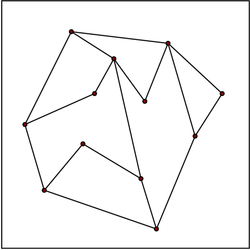
A planar subdivision inside a bounding box

In the planar case, we are given a planar subdivision S, formed by multiple polygons called faces, and need to determine which face contains a query point. A brute force search of each face using the point-in-polygon algorithm is possible, but usually not feasible for subdivisions of high complexity. Several different approaches lead to optimal data structures, with O(n) storage space and O(log n) query time, where n is the total number of vertices in S. For simplicity, we assume that the planar subdivision is contained inside a square bounding box.

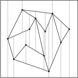
Slab decomposition

A planar subdivision divided into slabs.

The simplest and earliest data structure to achieve O(log n) time was discovered by Dobkin and Lipton in 1976. It is based on subdividing S using vertical lines that pass through each vertex in S. The region between two consecutive vertical lines is called a slab. Notice that each slab is divided by non-intersecting line segments that completely cross the slab from left to right. The region between two consecutive segments inside a slab corresponds to a unique face of S. Therefore, we reduce our point location problem to two simpler problems:

Given a subdivision of the plane into vertical slabs, determine which slab contains a given point.
Given a slab subdivided into regions by non-intersecting segments that completely cross the slab from left to right, determine which region contains a given point.

The first problem can be solved by binary search on the x coordinate of the vertical lines in O(log n) time. The second problem can also be solved in O(log n) time by binary search. To see how, notice that, as the segments do not intersect and completely cross the slab, the segments can be sorted vertically inside each slab.

While this algorithm allows point location in logarithmic time and is easy to implement, the space required to build the slabs and the regions contained within the slabs can be as high as O(n²), since each slab can cross a significant fraction of the segments.

Several authors noticed that the segments that cross two adjacent slabs are mostly the same. Therefore, the size of the data structure can be significantly reduced. More specifically, Snarak and Tarjan sweep a vertical line l from left to right over the plane, while maintaining the segments that intersect l in a Persistent red-black tree. This allows them to reduce the storage space to O(n), while maintaining the O(log n) query time.

Monotone subdivisions

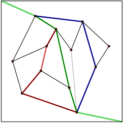
A monotone planar subdivision with some monotone chains highlighted.

A (vertical) monotone chain is a path such that the y-coordinate never increases along the path. A simple polygon is (vertical) monotone if it is formed by two monotone chains, with the first and last vertices in common. It is possible to add some edges to a planar subdivision, in order to make all faces monotone, obtaining what is called a monotone subdivision. This process does not add any vertices to the subdivision (therefore, the size remains O(n)), and can be performed in O(n log n) time by plane sweep (it can also be performed in linear time, using polygon triangulation). Therefore, there is no loss of generality, if we restrict our data structure to the case of monotone subdivisions, as we do in this section.

The weakness of the slab decomposition is that the vertical lines create additional segments in the decomposition, making it difficult to achieve O(n) storage space. Edelsbrunner, Guibas, and Stolfi discovered an optimal data structure that only uses the edges in a monotone subdivision. The idea is to use vertical monotone chains, instead of using vertical lines to partition the subdivision.

Converting this general idea to an actual efficient data structure is not a simple task. First, we need to be able to compute a monotone chain that divides the subdivision into two halves of similar sizes. Second, since some edges may be contained in several monotone chains, we need to be careful to guarantee that the storage space is O(n). Third, testing whether a point is on the left or the right side of a monotone subdivision takes O(n) time if performed naively.

Details on how to solve the first two issues are beyond the scope of this article. We briefly mention how to address the third issue. Using binary search, we can test whether a point is to the left or right of a monotone chain in O(log n) time. As we need to perform another nested binary search through O(log n) chains to actually determine the point location, the query time is O(log² n). To achieve O(log n) query time, we need to use fractional cascading, keeping pointers between the edges of different monotone chains.

Triangulation refinement

Successive steps of triangulation refinement.

A polygon with m vertices can be partitioned into m-2 triangles. There are numerous algorithms to triangulate a polygon efficiently, the fastest having O(n) worst case time. Therefore, we can decompose each polygon of our subdivision in triangles, and restrict our data structure to the case of subdivisions formed exclusively by triangles. Kirkpatrick gives a data structure for point location in triangulated subdivisions with O(n) storage space and O(log n) query time.

The general idea is to build a hierarchy of triangles. To perform a query, we start by finding the top-level triangle that contains the query point. Since the number of top-level triangles is bounded by a constant, this operation can be performed in O(1) time. Each triangle has pointers to the triangles it intersects in the next level of the hierarchy, and the number of pointers is also bounded by a constant. We proceed with the query by finding which triangle contains the query point level by level.

The data structure is built in the opposite order, that is, bottom-up. We start with the triangulated subdivision, and choose an independent set of vertices to be removed. After removing the vertices, we retriangulate the subdivision. Because the subdivision is formed by triangles, a greedy algorithm can find an independent set that contains a constant fraction of the vertices. Therefore, the number of removal steps is O(log n).

Trapezoidal decomposition

A trapezoidal decomposition.

A randomized approach to this problem, and probably the most practical one, is based on trapezoidal decomposition, or trapezoidal map. A trapezoidal decomposition is obtained by shooting vertical bullets going both up and down from each vertex in the original subdivision. The bullets stop when they hit an edge, and form a new edge in the subdivision. This way, we obtain a subset of the slab decomposition, with only O(n) edges and vertices, since we only add two edges and two vertices for each vertex in the original subdivision.

It is not easy to see how to use a trapezoidal decomposition for point location, since a binary search similar to the one used in the slab decomposition can no longer be performed. Instead, we need to answer a query in the same fashion as the triangulation refinement approach, but the data structure is constructed top-down. Initially, we build a trapezoidal decomposition containing only the bounding box, and no internal vertex. Then, we add the segments from the subdivision, one by one, in random order, refining the trapezoidal decomposition. Using backwards analysis, we can show that the expected number of trapezoids created for each insertion is bounded by a constant.

We build a directed acyclic graph, where the vertices are the trapezoids that existed at some point in the refinement, and the directed edges connect the trapezoids obtained by subdivision. The expected depth of a search in this digraph, starting from the vertex corresponding to the bounding box, is O(log n).

Higher dimensions

There are no known general point location data structures with linear space and logarithmic query time for dimensions greater than 2. Therefore, we need to sacrifice either query time, or storage space, or restrict ourselves to some less general type of subdivision.

In three-dimensional space, it is possible to answer point location queries in O(log² n) using O(n log n) space. The general idea is to maintain several planar point location data structures, corresponding to the intersection of the subdivision with n parallel planes that contain each subdivision vertex. A naive use of this idea would increase the storage space to O(n²). In the same fashion as in the slab decomposition, the similarity between consecutive data structures can be exploited in order to reduce the storage space to O(n log n), but the query time increases to O(log² n).

In d-dimensional space, point location can be solved by recursively projecting the faces into a (d-1)-dimensional space. While the query time is O(log n), the storage space can be as high as $O(n^{2^{d}})$ . The high complexity of the d-dimensional data structures led to the study of special types of subdivision.

One important example is the case of arrangements of hyperplanes. An arrangement of n hyperplanes defines O(n^d) cells, but point location can be performed in O(log n) time with O(n^d) space by using Chazelle's hierarchical cuttings.

Another special type of subdivision is called rectilinear (or orthogonal) subdivision. In a rectilinear subdivision, all edges are parallel to one of the d orthogonal axis. In this case, point location can be answered in O(log^d-1 n) time with O(n) space.

References

de Berg, Mark; van Kreveld, Marc; Overmars, Mark; Schwarzkopf, Otfried (2000). "Chapter 6: Point location". Computational Geometry (2nd revised ed.). Springer-Verlag. pp. 121–146. ISBN 3-540-65620-0.
Dobkin, David; Lipton, Richard J. (1976). "Multidimensional searching problems". SIAM Journal on Computing. 5 (2): 181–186. doi:10.1137/0205015.
Snoeyink, Jack (2004). "Chapter 34: "Point Location". In Goodman, Jacob E.; O'Rourke, Joseph. Handbook of Discrete and Computational Geometry (2nd ed.). Chapman & Hall/CRC. ISBN 1-58488-301-4.
Sarnak, Neil; Tarjan, Robert E. (1986). "Planar point location using persistent search trees". Communications of the ACM. 29 (7): 669–679. doi:10.1145/6138.6151.
Edelsbrunner, Herbert; Guibas, Leonidas J.; Stolfi, Jorge (1986). "Optimal point location in a monotone subdivision". SIAM Journal on Computing. 15 (2): 317–340. doi:10.1137/0215023.
Kirkpatrick, David G. (1983). "Optimal search in planar subdivisions". SIAM Journal on Computing. 12 (1): 28–35. doi:10.1137/0212002.

External links

Point-Location Source Repository at Stony Brook University
Point-Location Queries in CGAL, the Computational Geometry Algorithms Library

This article is issued from Wikipedia - version of the 9/22/2016. The text is available under the Creative Commons Attribution/Share Alike but additional terms may apply for the media files.