Quartic function
- This article is about the univariate quartic. For the bivariate quartic, see Quartic plane curve.
In algebra, a quartic function is a function of the form

where a is nonzero, which is defined by a polynomial of degree four, called quartic polynomial.
Sometimes the term biquadratic is used instead of quartic, but, usually, biquadratic function refers to a quadratic function of a square (or, equivalently, to the function defined by a quartic polynomial without terms of odd degree), having the form

A quartic equation, or equation of the fourth degree, is an equation that equates a quartic polynomial to zero, of the form

where a ≠ 0.
The derivative of a quartic function is a cubic function.
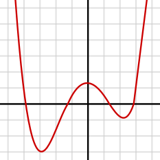
Since a quartic function is defined by a polynomial of even degree, it has the same infinite limit when the argument goes to positive or negative infinity. If a is positive, then the function increases to positive infinity at both ends; and thus the function has a global minimum. Likewise, if a is negative, it decreases to negative infinity and has a global maximum. In both cases it may or may not have another local maximum and another local minimum.
The degree four (quartic case) is the highest degree such that every polynomial equation can be solved by radicals.
History
Lodovico Ferrari is credited with the discovery of the solution to the quartic in 1540, but since this solution, like all algebraic solutions of the quartic, requires the solution of a cubic to be found, it could not be published immediately.[1] The solution of the quartic was published together with that of the cubic by Ferrari's mentor Gerolamo Cardano in the book Ars Magna.[2]
The Soviet historian I. Y. Depman claimed that even earlier, in 1486, Spanish mathematician Valmes was burned at the stake for claiming to have solved the quartic equation.[3] Inquisitor General Tomás de Torquemada allegedly told Valmes that it was the will of God that such a solution be inaccessible to human understanding.[4] However Beckmann, who popularized this story of Depman in the West, said that it was unreliable and hinted that it may have been invented as Soviet antireligious propaganda.[5] Beckmann's version of this story has been widely copied in several books and internet sites, usually without his reservations and sometimes with fanciful embellishments. Several attempts to find corroborating evidence for this story, or even for the existence of Valmes, have failed.[6]
The proof that four is the highest degree of a general polynomial for which such solutions can be found was first given in the Abel–Ruffini theorem in 1824, proving that all attempts at solving the higher order polynomials would be futile. The notes left by Évariste Galois prior to dying in a duel in 1832 later led to an elegant complete theory of the roots of polynomials, of which this theorem was one result.[7]
Applications
Each coordinate of the intersection points of two conic sections is a solution of a quartic equation. The same is true for the intersection of a line and a torus. It follows that quartic equations often arise in computational geometry and all related fields such as computer graphics, computer-aided design, computer-aided manufacturing and optics. Here are example of other geometric problems whose solution amounts of solving a quartic equation.
In computer-aided manufacturing, the torus is a shape that is commonly associated with the endmill cutter. To calculate its location relative to a triangulated surface, the position of a horizontal torus on the z-axis must be found where it is tangent to a fixed line, and this requires the solution of a general quartic equation to be calculated.
A quartic equation arises also in the process of solving the crossed ladders problem, in which the lengths of two crossed ladders, each based against one wall and leaning against another, are given along with the height at which they cross, and the distance between the walls is to be found.
In optics, Alhazen's problem is "Given a light source and a spherical mirror, find the point on the mirror where the light will be reflected to the eye of an observer." This leads to a quartic equation.[8][9][10]
Finding the distance of closest approach of two ellipses involves solving a quartic equation.
The eigenvalues of a 4×4 matrix are the roots of a quartic polynomial which is the characteristic polynomial of the matrix.
The characteristic equation of a fourth-order linear difference equation or differential equation is a quartic equation. An example arises in the Timoshenko-Rayleigh theory of beam bending.
Intersections between spheres, cylinders, or other quadrics can be found using quartic equations.
Inflection points and golden ratio
Letting F and G be the distinct inflection points of a quartic, and letting H be the intersection of the inflection secant line FG and the quartic, nearer to G than to F, then G divides FH into the golden section:[11]

Moreover, the area of the region between the secant line and the quartic below the secant line equals the area of the region between the secant line and the quartic above the secant line. One of those regions is disjointed into sub-regions of equal area.
Solving a quartic equation
Nature of the roots
Given the general quartic equation

with real coefficients and a ≠ 0 the nature of its roots is mainly determined by the sign of its discriminant

This may be refined by considering the signs of four other polynomials:

such that P/8a2 is the second degree coefficient of the associated depressed quartic (see below);

such that Q/8a3 is the first degree coefficient of the associated depressed quartic;

which is 0 if the quartic has a triple root; and

which is 0 if the quartic has two double roots.
The possible cases for the nature of the roots are as follows:[12]
- If ∆ < 0 then the equation has two distinct real roots and two complex conjugate non-real roots.
- If ∆ > 0 then either the equation's four roots are all real or none is.
- If P < 0 and D < 0 then all four roots are real and distinct.
- If P > 0 or D > 0 then there are two pairs of non-real complex conjugate roots.[13]
- If ∆ = 0 then (and only then) the polynomial has a multiple root. Here are the different cases that can occur:
- If P < 0 and D < 0 and ∆0 ≠ 0, there is a real double root and two real simple roots.
- If D > 0 or (P > 0 and (D ≠ 0 or Q ≠ 0)), there is a real double root and two complex conjugate roots.
- If ∆0 = 0 and D ≠ 0, there is a triple root and a simple root, all real.
- If D = 0, then:
- If P < 0, there are two real double roots.
- If P > 0 and Q = 0, there are two complex conjugate double roots.
- If ∆0 = 0, all four roots are equal to −b/4a
There are some cases that do not seem to be covered, but they cannot occur. For example, ∆0 > 0, P = 0 and D ≤ 0 is not one of the cases. However, if ∆0 > 0 and P = 0 then D > 0 so this combination is not possible.
General formula for roots

The four roots x1, x2, x3, and x4 for the general quartic equation

with a ≠ 0 are given in the following formula, which is deduced from the one in the section on Ferrari's method by back changing the variables (see section Converting to a depressed quartic) and using the formulas for the quadratic and cubic equations.

where p and q are the coefficients of the second and of the first degree respectively in the associated depressed quartic

and where
![{\displaystyle {\begin{aligned}S&={\frac {1}{2}}{\sqrt {-{\frac {2}{3}}\ p+{\frac {1}{3a}}\left(Q+{\frac {\Delta _{0}}{Q}}\right)}}\\Q&={\sqrt[{3}]{\frac {\Delta _{1}+{\sqrt {\Delta _{1}^{2}-4\Delta _{0}^{3}}}}{2}}}\end{aligned}}}](../I/m/a2123cde7bdf9a645323f6ccdc74817db4ddaf3b.svg)
(if S = 0 or Q = 0, see § Special cases of the formula, below)
with

and
- where is the aforementioned discriminant. For the cube root expression for Q, any of the three cube roots in the complex plane can be used, although if one of them is real that is the natural and simplest one to choose.The mathematical expressions of these last four terms are very similar to those of their cubic counterparts.


Special cases of the formula
- If the value of is a non-real complex number. In this case, either all roots are non-real or they are all real. In the latter case, the value of is also real, and one may prefer to express it in a purely real way, by using trigonometric functions, as follows:


- where


- If and the sign of has to be chosen to have that is one should define as maintaining the sign of
- If then one must change the choice of the cube root in in order to have This is always possible except if the quartic may be factored into The result is then correct, but misleading because it hides the fact that no cube root is needed in this case. In fact this case may occur only if the numerator of is zero, in which case the associated depressed quartic is biquadratic; it may thus be solved by the method described below.
- If and and thus also at least three roots are equal, and the roots are rational functions of the coefficients.
- If and the above expression for the roots is correct but misleading, hiding the fact that the polynomial is reducible and no cube root is needed to represent the roots.


Simpler cases
Reducible quartics
Consider the general quartic

It is reducible if Q(x) = R(x)×S(x), where R(x) and S(x) are non-constant polynomials with rational coefficients (or more generally with coefficients in the same field as the coefficients of Q(x)). There are two ways to write such a factorization: either

or

In either case, the roots of Q(x) are the roots of the factors, which may be computed by solving quadratic or cubic equations.
Detecting the existence of such factorizations can be done using the resolvent cubic of Q(x). It turns out that:
- if we are working over R (or, more generally, over some real closed field) then there is always such a factorization;
- if we are working over Q, then there is an algorithm to determine whether or not Q(x) is reducible and, if it is, how to express it as a product of polynomials of smaller degree.
In fact, several methods of solving quartic equations (Ferrari's method, Descartes' method, and, to a lesser extent, Euler's method) are based upon finding such factorizations.
Biquadratic equation
If a3 = a1 = 0 then the biquadratic function

defines a biquadratic equation, which is easy to solve.
Let z = x2. Then Q(x) becomes a quadratic q in z: q(z) = a4z2 + a2z + a0. Let z+ and z− be the roots of q(z). Then the roots of our quartic Q(x) are

Quasi-palindromic equation
The polynomial

is almost palindromic, as P(mx) = x4/m2P(m/x) (it is palindromic if m = 1). The change of variables z = x + m/x in P(x)/x2 = 0 produces the quadratic equation a0z2 + a1z + a2 − 2ma0 = 0. Since x2 − xz + m = 0, the quartic equation P(x) = 0 may be solved by applying the quadratic formula twice.
Solution methods
Converting to a depressed quartic
For solving purposes, it is generally better to convert the quartic into a depressed quartic by the following simple change of variable. All formulas are simpler and some methods work only in this case. The roots of the original quartic are easily recovered from that of the depressed quartic by the reverse change of variable.
Let

be the general quartic equation we want to solve.
Dividing by a4, provides the equivalent equation x4 + bx3 + cx2 + dx + e = 0, with b = a3/a4, c = a2/a4, d = a1/a4, and e = a0/a4. Substituting y − b/4 for x gives, after regrouping the terms, the equation y4 + py2 + qy + r = 0, where

If y0 is a root of this depressed quartic, then y0 − b/4 (that is y0 − a3/4a4) is a root of the original quartic and every root of the original quartic can be obtained by this process.
Ferrari's solution
As explained in the preceding section, we may start with the depressed quartic equation

This depressed quartic can be solved by means of a method discovered by Lodovico Ferrari. The depressed equation may be rewritten (this is easily verified by expanding the square and regrouping all terms in the left-hand side) as

Then, we introduce a variable m into the factor on the left-hand side by adding 2y2m + pm + m2 to both sides. After regrouping the coefficients of the power of y in the right-hand side, this gives the equation
-
(1)

which is equivalent to the original equation, whichever value is given to m.
As the value of m may be arbitrarily chosen, we will choose it in order to get a perfect square in the right-hand side. This implies that the discriminant in y of this quadratic equation is zero, that is m is a root of the equation

which may be rewritten as

This is the resolvent cubic of the quartic equation. The value of m may thus be obtained from Cardano's formula. When m is a root of this equation, the right-hand side of equation (1) is the square

However, this induces a division by zero if m = 0. This implies q = 0, and thus that the depressed equation is bi-quadratic, and may be solved by an easier method (see above). This was not a problem at the time of Ferrari, when one solved only explicitly given equations with numeric coefficients. For a general formula that is always true, one thus needs to choose a root of the cubic equation such that m ≠ 0. This is always possible except for the depressed equation x4 = 0.
Now, if m is a root of the cubic equation such that m ≠ 0, equation (1) becomes

This equation is of the form M 2 = N 2, which can be rearranged as M 2 − N 2 = 0 or (M + N)(M − N) = 0. Therefore, equation (1) may be rewritten as

This equation is easily solved by applying to each factor the quadratic formula. Solving them we may write the four roots as

where ±1 and ±2 denote either + or −. As the two occurrences of ±1 must denote the same sign, this leaves four possibilities, one for each root.
Therefore, the solutions of the original quartic equation are

A comparison with the general formula above shows that √2m = 2S.
Descartes' solution
Descartes[15] introduced in 1637 the method of finding the roots of a quartic polynomial by factoring it into two quadratic ones. Let

By equating coefficients, this results in the following system of equations:

This can be simplified by starting again with the depressed quartic y4 + py2 + qy + r, which can be obtained by substituting y − b/4 for x. Since the coefficient of y3 is 0, we get s = −u, and:

One can now eliminate both t and v by doing the following:
![{\displaystyle {\begin{aligned}u^{2}(p+u^{2})^{2}-q^{2}&=u^{2}(t+v)^{2}-u^{2}(t-v)^{2}\\&=u^{2}[(t+v+(t-v))(t+v-(t-v))]\\&=u^{2}(2t)(2v)\\&=4u^{2}tv\\&=4u^{2}r\end{aligned}}}](../I/m/3872dc7d07870b83c8d97f4fda44076625f066fe.svg)
If we set U = u2, then solving this equation becomes finding the roots of the resolvent cubic
-
U3 + 2pU2 + (p2 − 4r)U − q2,
(2)
which is done elsewhere. Then, if u is a square root of a non-zero root of this resolvent (such a non-zero root exists except for the quartic x4, which is trivially factored),

The symmetries in this solution are as follows. There are three roots of the cubic, corresponding to the three ways that a quartic can be factored into two quadratics, and choosing positive or negative values of u for the square root of U merely exchanges the two quadratics with one another.
The above solution shows that a quartic polynomial with rational coefficients and a zero coefficient on the cubic term is factorable into quadratics with rational coefficients if and only if either the resolvent cubic (2) has a non-zero root which is the square of a rational, or p2 − 4r is the square of rational and q = 0; this can readily be checked using the rational root test.[16]
Euler's solution
A variant of the previous method is due to Euler.[17][18] Unlike the previous methods, both of which use some root of the resolvent cubic, Euler's method uses all of them. Let us consider a depressed quartic x4 + px2 + qx + r. Observe that, if
- x4 + px2 + qx + r = (x2 + sx + t)(x2 − sx + v),
- r1 and r2 are the roots of x2 + sx + t,
- r3 and r4 are the roots of x2 − sx + v,
then
- the roots of x4 + px2 + qx + r are r1, r2, r3, and r4,
- r1 + r2 = −s,
- r3 + r4 = s.
Therefore, (r1 + r2)(r3 + r4) = −s2. In other words, −(r1 + r2)(r3 + r4) is one of the roots of the resolvent cubic (2) and this suggests that the roots of that cubic are equal to −(r1 + r2)(r3 + r4), −(r1 + r3)(r2 + r4), and −(r1 + r4)(r2 + r3). This is indeed true and it follows from Vieta's formulas. It also follows from Vieta's formulas, together with the fact that we are working with a depressed quartic, that r1 + r2 + r3 + r4 = 0. (Of course, this also follows from the fact that r1 + r2 + r3 + r4 = −s + s.) Therefore, if α, β, and γ are the roots of the resolvent cubic, then the numbers r1, r2, r3, and r4 are such that

It is a consequence of the first two equations that r1 + r2 is a square root of −α and that r3 + r4 is the other square root of −α. For the same reason,
- r1 + r3 is a square root of −β,
- r2 + r4 is the other square root of −β,
- r1 + r4 is a square root of −γ,
- r2 + r3 is the other square root of −γ.
Therefore, the numbers r1, r2, r3, and r4 are such that

the sign of the square roots will be dealt with below. The only solution of this system is:
![{\displaystyle \left\{{\begin{array}{l}r_{1}={\frac {{\sqrt {-\alpha }}+{\sqrt {-\beta }}+{\sqrt {-\gamma }}}{2}}\\[2mm]r_{2}={\frac {{\sqrt {-\alpha }}-{\sqrt {-\beta }}-{\sqrt {-\gamma }}}{2}}\\[2mm]r_{3}={\frac {-{\sqrt {-\alpha }}+{\sqrt {-\beta }}-{\sqrt {-\gamma }}}{2}}\\[2mm]r_{4}={\frac {-{\sqrt {-\alpha }}-{\sqrt {-\beta }}+{\sqrt {-\gamma }}}{2}}{\text{.}}\end{array}}\right.}](../I/m/59446e6989b84a9e543408589fa6d0663764bc97.svg)
Since, in general, there are two choices for each square root, it might look as if this provides 8 (= 23) choices for the set {r1, r2, r3, r4}, but, in fact, it provides no more than 2 such choices, because the consequence of replacing one of the square roots by the symmetric one is that the set {r1, r2, r3, r4} becomes the set {−r1, −r2, −r3, −r4}.
In order to determine the right sign of the square roots, one simply chooses some square root for each of the numbers −α, −β, and −γ and uses them to compute the numbers r1, r2, r3, and r4 from the previous equalities. Then, one computes the number √−α√−β√−γ. Note that, since α, β, and γ are the roots of (2), it is a consequence of Vieta's formulas that their product is equal to q2 and therefore that √−α√−β√−γ = ±q. But a straightforward computation shows that
- √−α√−β√−γ = r1r2r3 + r1r2r4 + r1r3r4 + r2r3r4.
If this number is −q, then the choice of the square roots was a good one (again, by Vieta's formulas); otherwise, the roots of the polynomial will be −r1, −r2, −r3, and −r4, which are the numbers obtained if one of the square roots is replaced by the symmetric one (or, what amounts to the same thing, if each of the three square roots is replaced by the symmetric one).
This argument suggests another way of choosing the square roots:
- pick any square root √−α of −α and any square root √−β of −β;
- define √−γ as .

Of course, this will make no sense if α or β is equal to 0, but 0 is a root of (2) only when q = 0, that is, only when we are dealing with a biquadratic equation, in which case there is a much simpler approach.
Solving by Lagrange resolvent
The symmetric group S4 on four elements has the Klein four-group as a normal subgroup. This suggests using a resolvent cubic whose roots may be variously described as a discrete Fourier transform or a Hadamard matrix transform of the roots; see Lagrange resolvents for the general method. Denote by xi, for i from 0 to 3, the four roots of x4 + bx3 + cx2 + dx + e. If we set

then since the transformation is an involution we may express the roots in terms of the four si in exactly the same way. Since we know the value s0 = −b/2, we only need the values for s1, s2 and s3. These are the roots of the polynomial

Substituting the si by their values in term of the xi, this polynomial may be expanded in a polynomial in s whose coefficients are symmetric polynomials in the xi. By the fundamental theorem of symmetric polynomials, these coefficients may be expressed as polynomials in the coefficients of the monic quartic. If, for simplification, we suppose that the quartic is depressed, that is b = 0, this results in the polynomial
-
(3)

This polynomial is of degree six, but only of degree three in s2, and so the corresponding equation is solvable by the method described in the article about cubic function. By substituting the roots in the expression of the xi in terms of the si, we obtain expression for the roots. In fact we obtain, apparently, several expressions, depending on the numbering of the roots of the cubic polynomial and of the signs given to their square roots. All these different expressions may be deduced from one of them by simply changing the numbering of the xi.
These expressions are unnecessarily complicated, involving the cubic roots of unity, which can be avoided as follows. If s is any non-zero root of (3), and if we set

then

We therefore can solve the quartic by solving for s and then solving for the roots of the two factors using the quadratic formula.
Note that this gives exactly the same formula for the roots as the one provided by Descartes' method.
Solving with algebraic geometry
There is an alternative solution using algebraic geometry[19] In brief, one interprets the roots as the intersection of two quadratic curves, then finds the three reducible quadratic curves (pairs of lines) that pass through these points (this corresponds to the resolvent cubic, the pairs of lines being the Lagrange resolvents), and then use these linear equations to solve the quadratic.
The four roots of the depressed quartic x4 + px2 + qx + r = 0 may also be expressed as the x coordinates of the intersections of the two quadratic equations y2 + py + qx + r = 0 and y − x2 = 0 i.e., using the substitution y = x2 that two quadratics intersect in four points is an instance of Bézout's theorem. Explicitly, the four points are Pi ≔ (xi, xi2) for the four roots xi of the quartic.
These four points are not collinear because they lie on the irreducible quadratic y = x2 and thus there is a 1-parameter family of quadratics (a pencil of curves) passing through these points. Writing the projectivization of the two quadratics as quadratic forms in three variables:

the pencil is given by the forms λF1 + μF2 for any point [λ, μ] in the projective line — in other words, where λ and μ are not both zero, and multiplying a quadratic form by a constant does not change its quadratic curve of zeros.
This pencil contains three reducible quadratics, each corresponding to a pair of lines, each passing through two of the four points, which can be done = 6 different ways. Denote these Q1 = L12 + L34, Q2 = L13 + L24, and Q3 = L14 + L23. Given any two of these, their intersection has exactly the four points.

The reducible quadratics, in turn, may be determined by expressing the quadratic form λF1 + μF2 as a 3×3 matrix: reducible quadratics correspond to this matrix being singular, which is equivalent to its determinant being zero, and the determinant is a homogeneous degree three polynomial in λ and μ and corresponds to the resolvent cubic.
See also
References
- ↑ O'Connor, John J.; Robertson, Edmund F., "Lodovico Ferrari", MacTutor History of Mathematics archive, University of St Andrews.
- ↑ Cardano, Gerolamo (1993) [1545], Ars magna or The Rules of Algebra, Dover, ISBN 0-486-67811-3
- ↑ Depman (1954), Rasskazy o matematike (in Russian), Leningrad: Gosdetizdat
- ↑ P. Beckmann (1971). A history of π. Macmillan. p. 80.
- ↑ P. Beckmann (1971). A history of π. Macmillan. p. 191.
- ↑ P. Zoll (1989). "Letter to the Editor". American Mathematical Monthly. 96 (8): 709–710. JSTOR 2324719.
- ↑ Stewart, Ian, Galois Theory, Third Edition (Chapman & Hall/CRC Mathematics, 2004)
- ↑ O'Connor, John J.; Robertson, Edmund F., "Abu Ali al-Hasan ibn al-Haytham", MacTutor History of Mathematics archive, University of St Andrews.
- ↑ MacKay, R. J.; Oldford, R. W. (August 2000), "Scientific Method, Statistical Method and the Speed of Light", Statistical Science, 15 (3): 254–78, doi:10.1214/ss/1009212817, MR 1847825
- ↑ Neumann, Peter M. (1998), "Reflections on Reflection in a Spherical Mirror", American Mathematical Monthly, 105 (6): 523−528, doi:10.2307/2589403, JSTOR 2589403
- ↑ Aude, H. T. R. (1949), "Notes on Quartic Curves", American Mathematical Monthly, 56 (3), doi:10.2307/2305030, JSTOR 2305030
- ↑ Rees, E. L. (1922). "Graphical Discussion of the Roots of a Quartic Equation". The American Mathematical Monthly. 29 (2): 51–55. doi:10.2307/2972804. JSTOR 2972804.
- ↑ Lazard, D. (1988). "Quantifier elimination: Optimal solution for two classical examples". Journal of Symbolic Computation. 5: 261–266. doi:10.1016/S0747-7171(88)80015-4.
- ↑ http://planetmath.org/QuarticFormula, PlanetMath, quartic formula, 21st October 2012
- ↑ Descartes, René (1954) [1637], "Book III: On the construction of solid and supersolid problems", The Geometry of Rene Descartes with a facsimile of the first edition, Dover, ISBN 0-486-60068-8, Zbl 51.0020.07
- ↑ Brookfield, G. (2007). "Factoring quartic polynomials: A lost art" (PDF). Mathematics Magazine. 80 (1): 67–70.
- ↑ van der Waerden, Bartel Leendert (1991), "The Galois theory: Equations of the second, third, and fourth degrees", Algebra, 1 (7th ed.), Springer-Verlag, ISBN 0-387-97424-5, Zbl 00048827
- ↑ Euler, Leonhard (1984) [1765], "Of a new method of resolving equations of the fourth degree", Elements of Algebra, Springer-Verlag, ISBN 978-1-4613-8511-0, Zbl 0557.01014
- ↑ Faucette, William M. (1996), "A Geometric Interpretation of the Solution of the General Quartic Polynomial", American Mathematical Monthly, 103 (1): 51–57, doi:10.2307/2975214, JSTOR 2975214, MR 1369151
Further reading
- Carpenter, W. (1966). "On the solution of the real quartic". Mathematics Magazine. 39: 28–30. doi:10.2307/2688990.
- Shmakov, S.L. (2011). "A Universal Method of Solving Quartic Equations" (PDF). International Journal of Pure and Applied Mathematics. 71: 251–259.