Solubility equilibrium

Solubility equilibrium is a type of dynamic equilibrium that exists when a chemical compound in the solid state is in chemical equilibrium with a solution of that compound. The solid may dissolve unchanged, with dissociation or with chemical reaction with another constituent of the solvent, such as acid or alkali. Each type of equilibrium is characterized by a temperature-dependent equilibrium constant. Solubility equilibria are important in pharmaceutical, environmental and many other scenarios.

Definitions

A solubility equilibrium exists when a chemical compound in the solid state is in chemical equilibrium with a solution of that compound. The equilibrium is an example of dynamic equilibrium in that some individual molecules migrate between the solid and solution phases such that the rates of dissolution and precipitation are equal to one another. When equilibrium is established, the solution is said to be saturated. The concentration of the solute in a saturated solution is known as the solubility. Units of solubility may be molar (mol dm⁻³) or expressed as mass per unit volume, such as μg ml⁻¹. Solubility is temperature dependent. A solution containing a higher concentration of solute than the solubility is said to be supersaturated. A supersaturated solution may be induced to come to equilibrium by the addition of a "seed" which may be a tiny crystal of the solute, or a tiny solid particle, which initiates precipitation.

There are three main types of solubility equilibria.

1. Simple dissolution.
2. Dissolution with dissociation. This is characteristic of salts. The equilibrium constant is known in this case as a solubility product.
3. Dissolution with reaction. This is characteristic of the dissolution of weak acids or weak bases in aqueous media of varying pH.

In each case an equilibrium constant can be specified as a quotient of activities. This equilibrium constant is dimensionless as activity is a dimensionless quantity. However, use of activities is very inconvenient, so the equilibrium constant is usually divided by the quotient of activity coefficients, to become a quotient of concentrations. See equilibrium chemistry#Equilibrium constant for details. Moreover, the concentration of solvent is usually taken to be constant and so is also subsumed into the equilibrium constant. For these reasons, the constant for a solubility equilibrium has dimensions related to the scale on which concentrations are measured. Solubility constants defined in terms of concentrations are not only temperature dependent, but also may depend on solvent composition when the solvent contains also species other than those derived from the solute.

Phase effect

Equilibria are defined for specific crystal phases. Therefore, the solubility product is expected to be different depending on the phase of the solid. For example, aragonite and calcite will have different solubility products even though they have both the same chemical identity (calcium carbonate). Under any given conditions one phase will be thermodynamically more stable than the other; therefore, this phase will form when thermodynamic equilibrium is established. However, kinetic factors may favor the formation the unfavorable precipitate (e.g. aragonite), which is then said to be in a metastable state.

Particle size effect

The thermodynamic solubility constant is defined for large monocrystals. Solubility will increase with decreasing size of solute particle (or droplet) because of the additional surface energy. This effect is generally small unless particles become very small, typically smaller than 1 μm. The effect of the particle size on solubility constant can be quantified as follows:

${\displaystyle \log(^{*}K_{A})=\log(^{*}K_{A\to 0})+{\frac {\gamma A_{\mathrm {m} }}{3.454RT}}}$

where *K_A is the solubility constant for the solute particles with the molar surface area A, *K_A→0 is the solubility constant for substance with molar surface area tending to zero (i.e., when the particles are large), γ is the surface tension of the solute particle in the solvent, A_m is the molar surface area of the solute (in m²/mol), R is the universal gas constant, and T is the absolute temperature.^[1]

Salt effect

The salt effect^[2] refers to the fact that the presence of a salt which has no ion in common with the solute, has an effect on the ionic strength of the solution and hence on activity coefficients, so that the equilibrium constant, expressed as a concentration quotient, changes.

Temperature effect

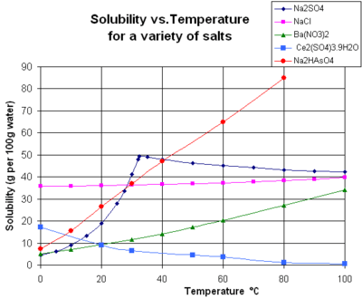
Solubility is sensitive to changes in temperature. For example, sugar is more soluble in hot water than cool water. It occurs because solubility constants, like other types of equilibrium constants, are functions of temperature. In accordance with Le Chatelier's Principle, when the dissolution process is endothermic (heat is absorbed), solubility increases with rising temperature. This effect is the basis for the process of recrystallization, which can be used to purify a chemical compound. When dissolution is exothermic (heat is released) solubility decreases with rising temperature.^[3] Sodium sulfate shows increasing solubility with temperature below about 32.4 °C, but a decreasing solubility at higher temperature.^[4] This is because the solid phase is the decahydrate (Na
2SO
4·10H
2O) below the transition temperature, but a different hydrate above that temperature.

Pressure effect

For condensed phases (solids and liquids), the pressure dependence of solubility is typically weak and usually neglected in practice. Assuming an ideal solution, the dependence can be quantified as:

${\displaystyle \left({\frac {\partial \ln N_{i}}{\partial P}}\right)_{T}=-{\frac {V_{i,\mathrm {aq} }-V_{i,\mathrm {cr} }}{RT}}}$

where the index i iterates the components, N_i is the mole fraction of the ith component in the solution, P is the pressure, the index T refers to constant temperature, V_i,aq is the partial molar volume of the ith component in the solution, V_i,cr is the partial molar volume of the ith component in the dissolving solid, and R is the universal gas constant.^[5]

The pressure dependence of solubility does occasionally have practical significance. For example, precipitation fouling of oil fields and wells by calcium sulfate (which decreases its solubility with decreasing pressure) can result in decreased productivity with time.

Simple dissolution

Dissolution of an organic solid can be described as an equilibrium between the substance in its solid and dissolved forms. For example, when sucrose (table sugar) forms a saturated solution

C₁₂H₂₂O₁₁(s) ⇌ C₁₂H₂₂O₁₁(aq).

An equilibrium expression for this reaction can be written, as for any chemical reaction (products over reactants):

${\displaystyle K^{\ominus }={\frac {\left\{\mathrm {{C}_{12}{H}_{22}{O}_{11}(aq)} \right\}}{\left\{\mathrm {{C}_{12}{H}_{22}{O}_{11}(s)} \right\}}}}$

where K^o is called the thermodynamic solubility constant. The braces indicate activity. The activity of a pure solid is, by definition, unity. Therefore

${\displaystyle K^{\ominus }=\left\{\mathrm {{C}_{12}{H}_{22}{O}_{11}(aq)} \right\}}$

The activity of a substance, A, in solution can be expressed as the product of the concentration, [A], and an activity coefficient, γ. When K^o is divided by γ, the solubility constant, K_s,

${\displaystyle K_{\mathrm {s} }=\left[\mathrm {{C}_{12}{H}_{22}{O}_{11}(aq)} \right]\,}$

is obtained. This is equivalent to defining the standard state as the saturated solution so that the activity coefficient is equal to one. The solubility constant is a true constant only if the activity coefficient is not affected by the presence of any other solutes that may be present. The unit of the solubility constant is the same as the unit of the concentration of the solute. For sucrose K = 1.971 mol dm⁻³ at 25 °C. This shows that the solubility of sucrose at 25 °C is nearly 2 mol dm⁻³ (540 g/l). Sucrose is unusual in that it does not easily form a supersaturated solution at higher concentrations, as do most other carbohydrates.

Dissolution with dissociation

Ionic compounds normally dissociate into their constituent ions when they dissolve in water. For example, for calcium sulfate:

CaSO₄(s) ⇌ Ca²⁺(aq) + SO2−
4(aq)

As for the previous example, the equilibrium expression is:

${\displaystyle K^{\ominus }={\frac {\left\{{\ce {Ca^{2+}(aq)}}\right\}\left\{{\ce {SO4^{2-}(aq)}}\right\}}{\left\{{\ce {CaSO4(s)}}\right\}}}=\left\{{\ce {Ca^{2+}(aq)}}\right\}\left\{{\ce {SO4^{2-}(aq)}}\right\}}$

where K^o is the thermodynamic equilibrium constant and braces indicate activity. The activity of a pure solid is, by definition, equal to one.

When the solubility of the salt is very low the activity coefficients of the ions in solution are nearly equal to one. By setting them to be actually equal to one this expression reduces to the solubility product expression:

${\displaystyle K_{\ce {sp}}=\left[{\ce {Ca^{2+}(aq)}}\right]\left[{\ce {SO4^{2-}(aq)}}\right].\,}$

The solubility product for a general binary compound A_pB_q is given by

A_pB_q ⇌ p A^q+ + q B^p−

K_sp = [A]^p[B]^q (electrical charges omitted for simplicity of notation)

When the product dissociates the concentration of B is equal to q/p times the concentration of A.

[B] = q/p[A]

Therefore

${\displaystyle K_{\ce {sp}}=[{\ce {A}}]^{p}\left({\frac {q}{p}}\right)^{q}[{\ce {A}}]^{q}=\left({\frac {q}{p}}\right)^{q}[{\ce {A}}]^{p+q}}$

${\displaystyle [{\ce {A}}]={\sqrt[{p+q}]{K_{\ce {sp}} \over {\left({\frac {q}{p}}\right)^{q}}}}}$

The solubility, S is 1/p[A]. One may incorporate 1/p and insert it under the root to obtain

${\displaystyle S={[{\ce {A}}] \over p}={[{\ce {B}}] \over q}={\sqrt[{p+q}]{K_{\ce {sp}} \over {\left({\frac {q}{p}}\right)^{q}}p^{p+q}}}={\sqrt[{p+q}]{K_{\ce {sp}} \over {q^{q}}p^{p}}}}$

Examples

CaSO4	p = 1	q = 1	S = √Ksp
Na2SO4	p = 2	q = 1	${\displaystyle S={\sqrt[{3}]{K_{\ce {sp}} \over 4}}}$
Al2(SO4)3	p = 2	q = 3	${\displaystyle S={\sqrt[{5}]{K_{\ce {sp}} \over 108}}}$

Solubility products are often expressed in logarithmic form. Thus, for calcium sulfate, K_sp = 4.93×10⁻⁵, log K_sp = −4.32. The smaller the value, or the more negative the log value, the lower the solubility.

Some salts are not fully dissociated in solution. Examples include MgSO₄, famously discovered by Manfred Eigen to be present in seawater as both an inner sphere complex and an outer sphere complex.^[6] The solubility of such salts is calculated by the method outlined in dissolution with reaction.

Hydroxides

For hydroxides solubility products are often given in a modified form, K*_sp, using hydrogen ion concentration in place of hydroxide ion concentration.^[7] The two concentrations are related by the self-ionization constant for water, K_w.

K_w = [H⁺][OH⁻]

For example,

Ca(OH)₂ ⇌ Ca²⁺ + 2 OH⁻

K_sp = [Ca²⁺][OH⁻]² = [Ca²⁺]K_w²[H⁺]⁻²

K*_sp = K_sp/K2
w = [Ca²⁺][H⁺]⁻²

log K_sp for Ca(OH)₂ is about −5 at ambient temperatures; log K*_sp = −5 + 2 × 14 = 23, approximately.

Common-ion effect

The common-ion effect is the effect of decreasing the solubility of one salt, when another salt, which has an ion in common with it, is also present. For example, the solubility of silver chloride, AgCl, is lowered when sodium chloride, a source of the common ion chloride, is added to a suspension of AgCl in water.^[8]

AgCl(s) ⇌ Ag⁺(aq) + Cl⁻(aq);      K_sp = [Ag⁺][Cl⁻]

The solubility, S, in the absence of a common ion can be calculated as follows. The concentrations [Ag⁺] and [Cl⁻] are equal because one mole of AgCl dissociates into one mole of Ag⁺ and one mole of Cl⁻. Let the concentration of [Ag⁺](aq) be denoted by x.

K_sp = x²;      S = x = √K_sp

K_sp for AgCl is equal to 1.77×10⁻¹⁰ mol² dm⁻⁶ at 25 °C, so the solubility is 1.33×10⁻⁵ mol dm⁻³.

Now suppose that sodium chloride is also present, at a concentration of 0.01 mol dm⁻³. The solubility, ignoring any possible effect of the sodium ions, is now calculated by

K_sp = x(0.01 + x)

This is a quadratic equation in x, which is also equal to the solubility.

x² + 0.01x − K_sp = 0

In the case of silver chloride x² is very much smaller than 0.01x, so this term can be ignored. Therefore

S = x = K_sp/0.01 = 1.77×10⁻⁸ mol dm⁻³,

a considerable reduction. In gravimetric analysis for silver, the reduction in solubility due to the common ion effect is used to ensure "complete" precipitation of AgCl.

Dissolution with reaction

When a concentrated solution of ammonia is added to a suspension of silver chloride dissolution occurs because a complex of Ag⁺ is formed

A typical reaction with dissolution involves a weak base, B, dissolving in an acidic aqueous solution.

B(s) + H⁺ (aq) ⇌ BH⁺ (aq)

This reaction is very important for pharmaceutical products.^[9] Dissolution of weak acids in alkaline media is similarly important.

H_nA(s) + OH⁻(aq) ⇌ H_n−1A⁻(aq) + H₂O

The uncharged molecule usually has lower solubility than the ionic form, so solubility depends on pH and the acid dissociation constant of the solute. The term "intrinsic solubility" is used to describe the solubility of the un-ionized form in the absence of acid or alkali.

Leaching of aluminium salts from rocks and soil by acid rain is another example of dissolution with reaction: alumino-silicates are bases which react with the acid to form soluble species, such as Al³⁺(aq).

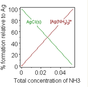
Formation of a chemical complex may also change solubility. A well-known example, is the addition of a concentrated solution of ammonia to a suspension of silver chloride, in which dissolution is favoured by the formation of an ammine complex.

AgCl(s) + 2 NH₃(aq) ⇌ [Ag(NH₃)₂]⁺(aq) + Cl⁻(aq)

Another example involves the addition of water softeners to washing powders to inhibit the precipitation of salts of magnesium and calcium ions, which are present in hard water, by forming complexes with them.

The calculation of solubility in these cases requires two or more simultaneous equilibria to be considered. For example,

Intrinsic solubility equilibrium	B(s) ⇌ B(aq)	Ks = [B(aq)]
Acid–base equilibrium	B(aq) + H^+(aq) ⇌ BH^+(aq)	Ka = [B(aq)][H^+(aq)]/[BH^+(aq)]

Experimental determination

The determination of solubility is fraught with difficulties.^[1] First and foremost is the difficulty in establishing that the system is in equilibrium at the chosen temperature. This is because both precipitation and dissolution reactions may be extremely slow. If the process is very slow solvent evaporation may be an issue. Supersaturation may occur. With very insoluble substances, the concentrations in solution are very low and difficult to determine. The methods used fall broadly into two categories, static and dynamic.

Static methods

In static methods a mixture is brought to equilibrium and the concentration of a species in the solution phase is determined by chemical analysis. This usually requires separation of the solid and solution phases. In order to do this the equilibration and separation should be performed in a thermostatted room.^[10] Very low concentrations can be measured if a radioactive tracer is incorporated in the solid phase.

A variation of the static method is to add a solution of the substance in a non-aqueous solvent, such as dimethyl sulfoxide, to an aqueous buffer mixture.^[11] Immediate precipitation may occur giving a cloudy mixture. The solubility measured for such a mixture is known as "kinetic solubility". The cloudiness is due to the fact that the precipitate particles are very small resulting in Tyndall scattering. In fact the particles are so small that the particle size effect comes into play and kinetic solubility is often greater than equilibrium solubility. Over time the cloudiness will disappear as the size of the crystallites increases, and eventually equilibrium will be reached in a process known as precipitate ageing.^[12]

Dynamic methods

Solubility values of organic acids, bases, and ampholytes of pharmaceutical interest may be obtained by a proceess called "Chasing equilibrium solubility".^[13] In this procedure, a quantity of substance is first dissolved at a pH where it exists predominantly in its ionized form and then a precipitate of the neutral (un-ionized) species is formed by changing the pH. Subsequently, the rate of change of pH due to precipitation or dissolution is monitored and strong acid and base titrant are added to adjust the pH to discover the equilibrium conditions when the two rates are equal. The advantage of this method is that it is relatively fast as the quantity of precipitate formed is quite small. However, the performance of the method may be affected by the formation supersaturated solutions.

See also

• Solubility table: A table of solubilities of mostly inorganic salts at temperatures between 0 and 100 °C.
• Molar solubility: The number of moles of a substance (the solute) that can be dissolved per liter of solution before the solution becomes saturated.
• Solvent models

References

1. Hefter, G. T.; Tomkins, R. P. T., eds. (2003). The Experimental Determination of Solubilities. Wiley-Blackwell. ISBN 0-471-49708-8.
2. Mendham, J.; Denney, R. C.; Barnes, J. D.; Thomas, M. J. K. (2000), Vogel's Quantitative Chemical Analysis (6th ed.), New York: Prentice Hall, ISBN 0-582-22628-7 Section 2.14
3. Pauling, Linus (1970). General Chemistry. Dover Publishing. p. 450.
4. Linke, W.F.; Seidell, A. (1965). Solubilities of Inorganic and Metal Organic Compounds (4th ed.). Van Nostrand. ISBN 0-8412-0097-1.
5. Gutman, E. M. (1994). Mechanochemistry of Solid Surfaces. World Scientific Publishing.
6. Eigen, Manfred (1967). "Nobel lecture" (PDF). Nobel Prize.
7. Baes, C. F.; Mesmer, R. E. (1976). The Hydrolysis of Cations. New York: Wiley.
8. Housecroft, C. E.; Sharpe, A. G. (2008). Inorganic Chemistry (3rd ed.). Prentice Hall. ISBN 978-0131755536. Section 6.10.
9. Payghan, Santosh (2008). "Potential Of Solubility In Drug Discovery And development". Pharminfo.net. Archived from the original on March 30, 2010. Retrieved 5 July 2010.
10. Rossotti, F. J. C.; Rossotti, H. (1961). "Chapter 9: Solubility". The Determination of Stability Constants. McGraw-Hill.
11. Aqueous solubility measurement – kinetic vs. thermodynamic methods Archived July 11, 2009, at the Wayback Machine.
12. Mendham, J.; Denney, R. C.; Barnes, J. D.; Thomas, M. J. K. (2000), Vogel's Quantitative Chemical Analysis (6th ed.), New York: Prentice Hall, ISBN 0-582-22628-7 Chapter 11: Gravimetric analysis
13. Stuart, M.; Box, K. (2005). "Chasing Equilibrium: Measuring the Intrinsic Solubility of Weak Acids and Bases". Anal. Chem. 77 (4): 983–990. doi:10.1021/ac048767n. PMID 15858976.

External links

• Housecroft, C. E.; Sharpe, A. G. (2008). Inorganic Chemistry (3rd ed.). Prentice Hall. ISBN 978-0131755536. Section 6.9: Solubilities of ionic salts. Includes a discussion of the thermodynamics of dissolution.
• IUPAC–NIST solubility database
• Solubility products of simple inorganic compounds
• Solubility challenge: Predict solubilities from a data base of 100 molecules. The database, of mostly compounds of pharmaceutical interest, is available at One hundred molecules with solubilities (Text file, tab separated).

A number of computer programs are available to do the calculations. They include:

• CHEMEQL: A comprehensive computer program for the calculation of thermodynamic equilibrium concentrations of species in homogeneous and heterogeneous systems. Many geochemical applications.
• JESS: All types of chemical equilibria can be modelled including protonation, complex formation, redox, solubility and adsorption interactions. Includes an extensive database.
• MINEQL+: A chemical equilibrium modeling system for aqueous systems. Handles a wide range of pH, redox, solubility and sorption scenarios.
• PHREEQC: USGS software designed to perform a wide variety of low-temperature aqueous geochemical calculations, including reactive transport in one dimension.
• MINTEQ: A chemical equilibrium model for the calculation of metal speciation, solubility equilibria etc. for natural waters.
• WinSGW: A Windows version of the SOLGASWATER computer program.