Checking whether a coin is fair
In statistics, the question of checking whether a coin is fair is one whose importance lies, firstly, in providing a simple problem on which to illustrate basic ideas of statistical inference and, secondly, in providing a simple problem that can be used to compare various competing methods of statistical inference, including decision theory. The practical problem of checking whether a coin is fair might be considered as easily solved by performing a sufficiently large number of trials, but statistics and probability theory can provide guidance on two types of question; specifically those of how many trials to undertake and of the accuracy an estimate of the probability of turning up heads, derived from a given sample of trials.
A fair coin is an idealized randomizing device with two states (usually named "heads" and "tails") which are equally likely to occur. It is based on the coin flip used widely in sports and other situations where it is required to give two parties the same chance of winning. Either a specially designed chip or more usually a simple currency coin is used, although the latter might be slightly "unfair" due to an asymmetrical weight distribution, which might cause one state to occur more frequently than the other, giving one party an unfair advantage.[1] So it might be necessary to test experimentally whether the coin is in fact "fair" – that is, whether the probability of the coin falling on either side when it is tossed is exactly 50%. It is of course impossible to rule out arbitrarily small deviations from fairness such as might be expected to affect only one flip in a lifetime of flipping; also it is always possible for an unfair (or "biased") coin to happen to turn up exactly 10 heads in 20 flips. As such, any fairness test must only establish a certain degree of confidence in a certain degree of fairness (a certain maximum bias). In more rigorous terminology, the problem is of determining the parameters of a Bernoulli process, given only a limited sample of Bernoulli trials.
Preamble
This article describes experimental procedures for determining whether a coin is fair or not fair. There are many statistical methods for analyzing such an experimental procedure. This article illustrates two of them.
Both methods prescribe an experiment (or trial) in which the coin is tossed many times and the result of each toss is recorded. The results can then be analysed statistically to decide whether the coin is "fair" or "probably not fair".
- Posterior probability density function, or PDF (Bayesian approach). The true probability of obtaining a particular side when a fair coin is tossed is unknown, but the uncertainty is initially represented by the "prior distribution". The theory of Bayesian inference is used to derive the posterior distribution by combining the prior distribution and the likelihood function which represents the information obtained from the experiment. The probability that this particular coin is a "fair coin" can then be obtained by integrating the PDF of the posterior distribution over the relevant interval that represents all the probabilities that can be counted as "fair" in a practical sense.
- Estimator of true probability (Frequentist approach). This method assumes that the experimenter can decide to toss the coin any number of times. He first decides on the level of confidence required and the tolerable margin of error. These parameters determine the minimum number of tosses that must be performed to complete the experiment.
An important difference between these two approaches is that the first approach gives some weight to one's prior experience of tossing coins, while the second does not. The question of how much weight to give to prior experience, depending on the quality (credibility) of that experience, is discussed under credibility theory.
Posterior probability density function
One method is to calculate the posterior probability density function of Bayesian probability theory.
A test is performed by tossing the coin N times and noting the observed numbers of heads, h, and tails, t. The symbols H and T represent more generalised variables expressing the numbers of heads and tails respectively that might have been observed in the experiment. Thus N = H+T = h+t.
Next, let r be the actual probability of obtaining heads in a single toss of the coin. This is the property of the coin which is being investigated. Using Bayes' theorem, the posterior probability density of r conditional on h and t is expressed as follows:

where g(r) represents the prior probability density distribution of r, which lies in the range 0 to 1.
The prior probability density distribution summarizes what is known about the distribution of r in the absence of any observation. We will assume that the prior distribution of r is uniform over the interval [0, 1]. That is, g(r) = 1. (In practice, it would be more appropriate to assume a prior distribution which is much more heavily weighted in the region around 0.5, to reflect our experience with real coins.)
The probability of obtaining h heads in N tosses of a coin with a probability of heads equal to r is given by the binomial distribution:

Substituting this into the previous formula:

This is in fact a beta distribution (the conjugate prior for the binomial distribution), whose denominator can be expressed in terms of the beta function:

As a uniform prior distribution has been assumed, and because h and t are integers, this can also be written in terms of factorials:

Example
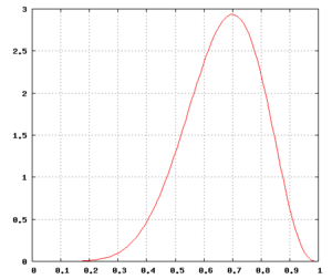
For example, let N = 10, h = 7, i.e. the coin is tossed 10 times and 7 heads are obtained:

The graph on the right shows the probability density function of r given that 7 heads were obtained in 10 tosses. (Note: r is the probability of obtaining heads when tossing the same coin once.)
The probability for an unbiased coin (defined for this purpose as one whose probability of coming down heads is somewhere between 45% and 55%)

is small when compared with the alternative hypothesis (a biased coin). However, it is not small enough to cause us to believe that the coin has a significant bias. Notice that this probability is slightly higher than our presupposition of the probability that the coin was fair corresponding to the uniform prior distribution, which was 10%. Using a prior distribution that reflects our prior knowledge of what a coin is and how it acts, the posterior distribution would not favor the hypothesis of bias. However the number of trials in this example (10 tosses) is very small, and with more trials the choice of prior distribution would be somewhat less relevant.)
Note that, with the uniform prior, the posterior probability distribution f(r | H = 7,T = 3) achieves its peak at r = h / (h + t) = 0.7; this value is called the maximum a posteriori (MAP) estimate of r. Also with the uniform prior, the expected value of r under the posterior distribution is
![\operatorname {E} [r]=\int _{0}^{1}r\cdot f(r|H=7,T=3)\,\mathrm {d} r={\frac {h+1}{h+t+2}}={\frac {2}{3}}\,.](../I/m/0ca1515e1432d24add2b96c7c4faca5c476d8e9b.svg)
Estimator of true probability
| The best estimator for the actual value is the estimator .
This estimator has a margin of error (E) where at a particular confidence level. |


Using this approach, to decide the number of times the coin should be tossed, two parameters are required:
- The confidence level which is denoted by confidence interval (Z)
- The maximum (acceptable) error (E)
- The confidence level is denoted by Z and is given by the Z-value of a standard normal distribution. This value can be read off a standard score statistics table for the normal distribution. Some examples are:
| Z value | Confidence Level | Comment |
|---|---|---|
| 0.6745 | gives 50.000% level of confidence | Half |
| 1.0000 | gives 68.269% level of confidence | One std dev |
| 1.6449 | gives 90.000% level of confidence | "One Nine" |
| 1.9599 | gives 95.000% level of confidence | 95 percent |
| 2.0000 | gives 95.450% level of confidence | Two std dev |
| 2.5759 | gives 99.000% level of confidence | "Two Nines" |
| 3.0000 | gives 99.730% level of confidence | Three std dev |
| 3.2905 | gives 99.900% level of confidence | "Three Nines" |
| 3.8906 | gives 99.990% level of confidence | "Four Nines" |
| 4.0000 | gives 99.993% level of confidence | Four std dev |
| 4.4172 | gives 99.999% level of confidence | "Five Nines" |
- The maximum error (E) is defined by where is the estimated probability of obtaining heads. Note: is the same actual probability (of obtaining heads) as of the previous section in this article.
- In statistics, the estimate of a proportion of a sample (denoted by p) has a standard error (standard deviation of error) given by:


where n is the number of trials (which was denoted by N in the previous section).
This standard error function of p has a maximum at . Further, in the case of a coin being tossed, it is likely that p will be not far from 0.5, so it is reasonable to take p=0.5 in the following:


And hence the value of maximum error (E) is given by

Solving for the required number of coin tosses, n,

Examples
1. If a maximum error of 0.01 is desired, how many times should the coin be tossed?

- at 68.27% level of confidence (Z=1)
- at 95.45% level of confidence (Z=2)
- at 99.90% level of confidence (Z=3.3)


2. If the coin is tossed 10000 times, what is the maximum error of the estimator on the value of (the actual probability of obtaining heads in a coin toss)?
- at 68.27% level of confidence (Z=1)
- at 95.45% level of confidence (Z=2)
- at 99.90% level of confidence (Z=3.3)


3. The coin is tossed 12000 times with a result of 5961 heads (and 6039 tails). What interval does the value of (the true probability of obtaining heads) lie within if a confidence level of 99.999% is desired?

Now find the value of Z corresponding to 99.999% level of confidence.

Now calculate E

The interval which contains r is thus:


Hence, 99.999% of the time, the interval above would contain which is the true value of obtaining heads in a single toss.
Other approaches
Other approaches to the question of checking whether a coin is fair are available using decision theory, whose application would require the formulation of a loss function or utility function which describes the consequences of making a given decision. An approach that avoids requiring either a loss function or a prior probability (as in the Bayesian approach) is that of "acceptance sampling".[2]
Other applications
The above mathematical analysis for determining if a coin is fair can also be applied to other uses. For example:
- Determining the proportion of defective items for a product subjected to a particular (but well defined) condition. Sometimes a product can be very difficult or expensive to produce. Furthermore, if testing such products will result in their destruction, a minimum number of items should be tested. Using a similar analysis, the probability density function of the product defect rate can be found.
- Two party polling. If a small random sample poll is taken where there are only two mutually exclusive choices, then this is similar to tossing a single coin multiple times using a possibly biased coin. A similar analysis can therefore be applied to determine the confidence to be ascribed to the actual ratio of votes cast. (Note that if people are allowed to abstain then the analysis must take account of that, and the coin-flip analogy doesn't quite hold.)
- Determining the sex ratio in a large group of an animal species. Provided that a small random sample (i.e. small in comparison with the total population) is taken when performing the random sampling of the population, the analysis is similar to determining the probability of obtaining heads in a coin toss.
See also
- Binomial test
- Coin flipping
- Confidence interval
- Estimation theory
- Inferential statistics
- Loaded dice
- Margin of error
- Point estimation
- Statistical randomness
References
- ↑ However, if the coin is caught rather than allowed to bounce or spin, it is difficult to bias a coin flip's outcome. See Gelman, Andrew; Deborah Nolan (2002). "Teacher's Corner: You Can Load a Die, But You Can't Bias a Coin". American Statistician. 56: 308–311. doi:10.1198/000313002605.
- ↑ Cox, D.R., Hinkley, D.V. (1974) Theoretical Statistics (Example 11.7), Chapman & Hall. ISBN 0-412-12420-3
- Guttman, Wilks, and Hunter: Introductory Engineering Statistics, John Wiley & Sons, Inc. (1971) ISBN 0-471-33770-6
- Devinder Sivia: Data Analysis, a Bayesian Tutorial, Oxford University Press (1996) ISBN 0-19-851889-7