Levenberg–Marquardt algorithm
In mathematics and computing, the Levenberg–Marquardt algorithm (LMA), also known as the damped least-squares (DLS) method, is used to solve non-linear least squares problems. These minimization problems arise especially in least squares curve fitting.
The LMA is used in many software applications for solving generic curve-fitting problems. However, as for many fitting algorithms, the LMA finds only a local minimum, which is not necessarily the global minimum. The LMA interpolates between the Gauss–Newton algorithm (GNA) and the method of gradient descent. The LMA is more robust than the GNA, which means that in many cases it finds a solution even if it starts very far off the final minimum. For well-behaved functions and reasonable starting parameters, the LMA tends to be a bit slower than the GNA. LMA can also be viewed as Gauss–Newton using a trust region approach.
The algorithm was first published in 1944 by Kenneth Levenberg,[1] while working at the Frankford Army Arsenal. It was rediscovered in 1963 by Donald Marquardt[2] who worked as a statistician at DuPont and independently by Girard,[3] Wynne[4] and Morrison.[5]
The problem
The primary application of the Levenberg–Marquardt algorithm is in the least-squares curve fitting problem: given a set of empirical datum pairs (xi, yi) of independent and dependent variables, find the parameters β of the model curve f(x, β) so that the sum of the squares of the deviations is minimized:

![{\displaystyle {\hat {\beta }}=\operatorname {argmin} \limits _{\beta }S(\beta )\equiv \operatorname {argmin} \limits _{\beta }\sum _{i=1}^{m}[y_{i}-f(x_{i},{\boldsymbol {\beta }})]^{2}.}](../I/m/84e2b0804af8425b72d8401ff98d573502faa243.svg)
The solution
Like other numeric minimization algorithms, the Levenberg–Marquardt algorithm is an iterative procedure. To start a minimization, the user has to provide an initial guess for the parameter vector, β. In cases with only one minimum, an uninformed standard guess like βT = (1, 1, ..., 1) will work fine; in cases with multiple minima, the algorithm converges to the global minimum only if the initial guess is already somewhat close to the final solution.
In each iteration step, the parameter vector β is replaced by a new estimate β + δ. To determine δ, the functions are approximated by their linearizations:


where

is the gradient (row-vector in this case) of f with respect to β.
The sum of squares at its minimum has a zero gradient with respect to β. The above first-order approximation of gives


or in vector notation,
![{\displaystyle {\begin{aligned}S({\boldsymbol {\beta }}+{\boldsymbol {\delta }})&\approx \|\mathbf {y} -\mathbf {f} ({\boldsymbol {\beta }})-\mathbf {J} {\boldsymbol {\delta }}\|^{2}\\&=[\mathbf {y} -\mathbf {f} ({\boldsymbol {\beta }})-\mathbf {J} {\boldsymbol {\delta }}]^{T}[\mathbf {y} -\mathbf {f} ({\boldsymbol {\beta }})-\mathbf {J} {\boldsymbol {\delta }}]\\&=[\mathbf {y} -\mathbf {f} ({\boldsymbol {\beta }})]^{T}[\mathbf {y} -\mathbf {f} ({\boldsymbol {\beta }})]-[\mathbf {y} -\mathbf {f} ({\boldsymbol {\beta }})]^{T}\mathbf {J} {\boldsymbol {\delta }}-(\mathbf {J} {\boldsymbol {\delta }})^{T}[\mathbf {y} -\mathbf {f} ({\boldsymbol {\beta }})]+{\boldsymbol {\delta }}^{T}\mathbf {J} ^{T}\mathbf {J} {\boldsymbol {\delta }}\\&=[\mathbf {y} -\mathbf {f} ({\boldsymbol {\beta }})]^{T}[\mathbf {y} -\mathbf {f} ({\boldsymbol {\beta }})]-2[\mathbf {y} -\mathbf {f} ({\boldsymbol {\beta }})]^{T}\mathbf {J} {\boldsymbol {\delta }}+{\boldsymbol {\delta }}^{T}\mathbf {J} ^{T}\mathbf {J} {\boldsymbol {\delta }}.\end{aligned}}}](../I/m/c94ad17f223c0ed1ca9efea02c7b8c3d2ee8d95d.svg)
Taking the derivative of with respect to δ and setting the result to zero gives

![{\displaystyle (\mathbf {J} ^{T}\mathbf {J} ){\boldsymbol {\delta }}=\mathbf {J} ^{T}[\mathbf {y} -f({\boldsymbol {\beta }})],}](../I/m/f1d128a1b6d24220f3fb47c227b78d84977a3acf.svg)
where is the Jacobian matrix whose i-th row equals , and where and are vectors with i-th component and respectively. This is a set of linear equations, which can be solved for δ.


Levenberg's contribution is to replace this equation by a "damped version",
![{\displaystyle (\mathbf {J} ^{T}\mathbf {J} +\lambda \mathbf {I} ){\boldsymbol {\delta }}=\mathbf {J} ^{T}[\mathbf {y} -\mathbf {f} ({\boldsymbol {\beta }})],}](../I/m/3c80c1b3179c3471f2bb000429150e16926a8bac.svg)
where I is the identity matrix, giving as the increment δ to the estimated parameter vector β.
The (non-negative) damping factor λ is adjusted at each iteration. If reduction of S is rapid, a smaller value can be used, bringing the algorithm closer to the Gauss–Newton algorithm, whereas if an iteration gives insufficient reduction in the residual, λ can be increased, giving a step closer to the gradient-descent direction. Note that the gradient of S with respect to δ equals . Therefore, for large values of λ, the step will be taken approximately in the direction of the gradient. If either the length of the calculated step δ or the reduction of sum of squares from the latest parameter vector β + δ fall below predefined limits, iteration stops, and the last parameter vector β is considered to be the solution.
![{\displaystyle -2{\big (}\mathbf {J} ^{T}[\mathbf {y} -\mathbf {f} ({\boldsymbol {\beta }})]{\big )}^{T}}](../I/m/dfe0694b8c2542f8c33f9a355ca148a74583ba68.svg)
Levenberg's algorithm has the disadvantage that if the value of damping factor λ is large, inverting JTJ + λI is not used at all. Marquardt provided the insight that we can scale each component of the gradient according to the curvature, so that there is larger movement along the directions where the gradient is smaller. This avoids slow convergence in the direction of small gradient. Therefore, Marquardt replaced the identity matrix I with the diagonal matrix consisting of the diagonal elements of JTJ, resulting in the Levenberg–Marquardt algorithm:
![{\displaystyle [\mathbf {J} ^{T}\mathbf {J} +\lambda \operatorname {diag} (\mathbf {J} ^{T}\mathbf {J} )]{\boldsymbol {\delta }}=\mathbf {J} ^{T}[\mathbf {y} -\mathbf {f} ({\boldsymbol {\beta }})].}](../I/m/6923eb0f097d41df2e71063644b2286e3bb27a83.svg)
A similar damping factor appears in Tikhonov regularization, which is used to solve linear ill-posed problems, as well as in ridge regression, an estimation technique in statistics.
Choice of damping parameter
Various more or less heuristic arguments have been put forward for the best choice for the damping parameter λ. Theoretical arguments exist showing why some of these choices guarantee local convergence of the algorithm; however, these choices can make the global convergence of the algorithm suffer from the undesirable properties of steepest descent, in particular very slow convergence close to the optimum.
The absolute values of any choice depends on how well-scaled the initial problem is. Marquardt recommended starting with a value λ0 and a factor ν > 1. Initially setting λ = λ0 and computing the residual sum of squares S(β) after one step from the starting point with the damping factor of λ = λ0 and secondly with λ0/ν. If both of these are worse than the initial point, then the damping is increased by successive multiplication by ν until a better point is found with a new damping factor of λ0νk for some k.
If use of the damping factor λ/ν results in a reduction in squared residual, then this is taken as the new value of λ (and the new optimum location is taken as that obtained with this damping factor) and the process continues; if using λ/ν resulted in a worse residual, but using λ resulted in a better residual, then λ is left unchanged and the new optimum is taken as the value obtained with λ as damping factor.
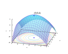
Example
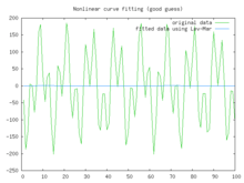


In this example we try to fit the function using the Levenberg–Marquardt algorithm implemented in GNU Octave as the leasqr function. The graphs show progressively better fitting for the parameters a = 100, b = 102 used in the initial curve. Only when the parameters in the last graph are chosen closest to the original, are the curves fitting exactly. This equation is an example of very sensitive initial conditions for the Levenberg–Marquardt algorithm. One reason for this sensitivity is the existence of multiple minima — the function has minima at parameter value and .


See also
- Trust region
- Nelder–Mead method (aka simplex)
- Variants of the Levenberg–Marquardt algorithm have also been used for solving nonlinear systems of equations.[6]
References
- ↑ Levenberg, Kenneth (1944). "A Method for the Solution of Certain Non-Linear Problems in Least Squares". Quarterly of Applied Mathematics. 2: 164–168.
- ↑ Marquardt, Donald (1963). "An Algorithm for Least-Squares Estimation of Nonlinear Parameters". SIAM Journal on Applied Mathematics. 11 (2): 431–441. doi:10.1137/0111030.
- ↑ Girard, André (1958). "Excerpt from Revue d'optique théorique et instrumentale". Rev. Opt. 37: 225–241, 397–424.
- ↑ Wynne, C. G. (1959). "Lens Designing by Electronic Digital Computer: I". Proc. Phys. Soc. London. 73 (5): 777. doi:10.1088/0370-1328/73/5/310.
- ↑ Morrison, David D. (1960). "Methods for nonlinear least squares problems and convergence proofs". Proceedings of the Jet Propulsion Laboratory Seminar on Tracking Programs and Orbit Determination: 1–9.
- ↑ Christian Kanzow, Nobuo Yamashita, Masao Fukushima: "Levenberg-Marquardt methods with strong local convergence properties for solving nonlinear equations with convex constraints," JCAM, 172(2):375-97, Dec. 2004, DOI: 10.1016/j.cam.2004.02.013.
Additional reading
- Moré, Jorge J.; Sorensen, Daniel C. (1983). "Computing a Trust-Region Step". SIAM J. Sci. Stat. Comput. (4): 553–572.
- Gill, Philip E.; Murray, Walter (1978). "Algorithms for the solution of the nonlinear least-squares problem". SIAM Journal on Numerical Analysis. 15 (5): 977–992. doi:10.1137/0715063.
- Pujol, Jose (2007). "The solution of nonlinear inverse problems and the Levenberg-Marquardt method". Geophysics. SEG. 72 (4): W1–W16. doi:10.1190/1.2732552.
- Nocedal, Jorge; Wright, Stephen J. (2006). Numerical Optimization (2nd ed.). Springer. ISBN 0-387-30303-0.
External links
Descriptions
- Detailed description of the algorithm can be found in Numerical Recipes in C, Chapter 15.5: Nonlinear models
- C. T. Kelley, Iterative Methods for Optimization, SIAM Frontiers in Applied Mathematics, no 18, 1999, ISBN 0-89871-433-8. Online copy
- History of the algorithm in SIAM news
- A tutorial by Ananth Ranganathan
- Methods for Non-Linear Least Squares Problems by K. Madsen, H.B. Nielsen, O. Tingleff is a tutorial discussing non-linear least-squares in general and the Levenberg-Marquardt method in particular
- T. Strutz: Data Fitting and Uncertainty (A practical introduction to weighted least squares and beyond). 2nd edition, Springer Vieweg, 2016, ISBN 978-3-658-11455-8.
- H. P. Gavin, The Levenberg-Marquardt method for nonlinear least squares curve-fitting problems (MATLAB implementation included)
Implementations
- Levenberg-Marquardt is a built-in algorithm in Mathematica , Matlab, NeuroSolutions, GNU Octave, Origin, SciPy, Fityk, IGOR Pro and LabVIEW.
- The oldest implementation still in use is lmdif, from MINPACK, in Fortran, in the public domain. See also:
- lmfit, a self-contained C implementation of the MINPACK algorithm, with an easy-to-use wrapper for curve fitting, liberal licence (freeBSD).
- eigen, a C++ linear algebra library, includes an adaptation of the minpack algorithm in the "NonLinearOptimization" module.
- The GNU Scientific Library has a C interface to MINPACK.
- C/C++ Minpack includes the Levenberg–Marquardt algorithm.
- Several high-level languages and mathematical packages have wrappers for the MINPACK routines, among them:
- Python library scipy, module
scipy.optimize.leastsq, - IDL, add-on MPFIT.
- R (programming language) has the minpack.lm package.
- Python library scipy, module
- levmar is an implementation in C/C++ with support for constraints, distributed under the GNU General Public License.
- levmar includes a MEX file interface for MATLAB
- Perl (PDL), python, Haskell and .NET interfaces to levmar are available: see PDL::Fit::Levmar or PDL::Fit::LM, PyLevmar, HackageDB levmar and LevmarSharp.
- sparseLM is a C implementation aimed at minimizing functions with large, arbitrarily sparse Jacobians. Includes a MATLAB MEX interface.
- SMarquardt.m is a stand-alone routine for Matlab or Octave.
- InMin library contains a C++ implementation of the algorithm based on the eigen C++ linear algebra library. It has a pure C-language API as well as a Python binding
- ceres is a non-linear minimisation library with an implementation of the Levenberg–Marquardt algorithm. It is written in C++ and uses eigen
- ALGLIB has implementations of improved LMA in C# / C++ / Delphi / Visual Basic. Improved algorithm takes less time to converge and can use either Jacobian or exact Hessian.
- NMath has an implementation for the .NET Framework.
- gnuplot uses its own implementation gnuplot.info.
- Java programming language implementations: 1) Javanumerics, 2) LMA-package (a small, user friendly and well documented implementation with examples and support), 3) Apache Commons Math
- OOoConv implements the L-M algorithm as an OpenOffice.org Calc spreadsheet.
- SAS, there are multiple ways to access SAS's implementation of the Levenberg–Marquardt algorithm: it can be accessed via NLPLM Call in PROC IML and it can also be accessed through the LSQ statement in PROC NLP, and the METHOD=MARQUARDT option in PROC NLIN.
- LMAM/OLMAM Matlab toolbox implements Levenberg-Marquardt with adaptive momentum for training feedforward neural networks.
- GADfit is a Fortran implementation of global fitting based on a modified Levenberg-Marquardt. Uses automatic differentiation. Allows fitting functions of arbitrary complexity, including integrals.
- Artelys Knitro is a non-linear solver with an implementation of the Levenberg–Marquardt algorithm. It is written in C and has interfaces to C++/C#/Java/Python/MATLAB/R.
|  | |||||||||||||||||||||||||||
|
| ||||||||||||||||||||||||||||
| ||||||||||||||||||||||||||||
| ||||||||||||||||||||||||||||