Kriging
In statistics, originally in geostatistics, Kriging or Gaussian process regression is a method of interpolation for which the interpolated values are modeled by a Gaussian process governed by prior covariances, as opposed to a piecewise-polynomial spline chosen to optimize smoothness of the fitted values. Under suitable assumptions on the priors, Kriging gives the best linear unbiased prediction of the intermediate values. Interpolating methods based on other criteria such as smoothness need not yield the most likely intermediate values. The method is widely used in the domain of spatial analysis and computer experiments. The technique is also known as Wiener–Kolmogorov prediction, after Norbert Wiener and Andrey Kolmogorov.
The theoretical basis for the method was developed by the French mathematician Georges Matheron based on the Master's thesis of Danie G. Krige, the pioneering plotter of distance-weighted average gold grades at the Witwatersrand reef complex in South Africa. Krige sought to estimate the most likely distribution of gold based on samples from a few boreholes. The English verb is to krige and the most common noun is Kriging; both are often pronounced with a hard "g", following the pronunciation of the name "Krige".
Main principles
Related terms and techniques
The basic idea of Kriging is to predict the value of a function at a given point by computing a weighted average of the known values of the function in the neighborhood of the point. The method is mathematically closely related to regression analysis. Both theories derive a best linear unbiased estimator, based on assumptions on covariances, make use of Gauss-Markov theorem to prove independence of the estimate and error, and make use of very similar formulae. Even so, they are useful in different frameworks: Kriging is made for estimation of a single realization of a random field, while regression models are based on multiple observations of a multivariate data set.
The Kriging estimation may also be seen as a spline in a reproducing kernel Hilbert space, with the reproducing kernel given by the covariance function.[1] The difference with the classical Kriging approach is provided by the interpretation: while the spline is motivated by a minimum norm interpolation based on a Hilbert space structure, Kriging is motivated by an expected squared prediction error based on a stochastic model.
Kriging with polynomial trend surfaces is mathematically identical to generalized least squares polynomial curve fitting.
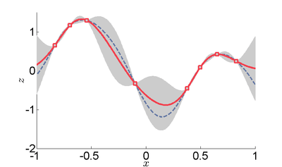
Kriging can also be understood as a form of Bayesian inference.[2] Kriging starts with a prior distribution over functions. This prior takes the form of a Gaussian process: samples from a function will be normally distributed, where the covariance between any two samples is the covariance function (or kernel) of the Gaussian process evaluated at the spatial location of two points. A set of values is then observed, each value associated with a spatial location. Now, a new value can be predicted at any new spatial location, by combining the Gaussian prior with a Gaussian likelihood function for each of the observed values. The resulting posterior distribution is also Gaussian, with a mean and covariance that can be simply computed from the observed values, their variance, and the kernel matrix derived from the prior.

Geostatistical estimator
In geostatistical models, sampled data is interpreted as the result of a random process. The fact that these models incorporate uncertainty in their conceptualization doesn't mean that the phenomenon - the forest, the aquifer, the mineral deposit - has resulted from a random process, but rather it allows one to build a methodological basis for the spatial inference of quantities in unobserved locations, and to quantify the uncertainty associated with the estimator.
A stochastic process is, in the context of this model, simply a way to approach the set of data collected from the samples. The first step in geostatistical modulation is to create a random process that best describes the set of observed data.
A value from location (generic denomination of a set of geographic coordinates) is interpreted as a realization of the random variable . In the space , where the set of samples is dispersed, there are realizations of the random variables , correlated between themselves.


The set of random variables constitutes a random function of which only one realization is known - the set of observed data. With only one realization of each random variable it's theoretically impossible to determine any statistical parameter of the individual variables or the function.

- The proposed solution in the geostatistical formalism consists in assuming various degrees of stationarity in the random function, in order to make possible the inference of some statistic values.
For instance, if one assumes, based on the homogeneity of samples in area where the variable is distributed, the hypothesis that the first moment is stationary (i.e. all random variables have the same mean), then one is assuming that the mean can be estimated by the arithmetic mean of sampled values. Judging such a hypothesis as appropriate is equivalent to considering the sample values sufficiently homogeneous to validate that representation.
The hypothesis of stationarity related to the second moment is defined in the following way: the correlation between two random variables solely depends on the spatial distance between them, and is independent of their location:


where

This hypothesis allows one to infer those two measures - the variogram and the covariogram - based on the samples:


where

Linear estimation
Spatial inference, or estimation, of a quantity , at an unobserved location , is calculated from a linear combination of the observed values and weights :


The weights are intended to summarize two extremely important procedures in a spatial inference process:

- reflect the structural "proximity" of samples to the estimation location,
- at the same time, they should have a desegregation effect, in order to avoid bias caused by eventual sample clusters
When calculating the weights , there are two objectives in the geostatistical formalism: unbias and minimal variance of estimation.
If the cloud of real values is plotted against the estimated values , the criterion for global unbias, intrinsic stationarity or wide sense stationarity of the field, implies that the mean of the estimations must be equal to mean of the real values.


The second criterion says that the mean of the squared deviations must be minimal, which means that when the cloud of estimated values versus the cloud real values is more disperse, the estimator is more imprecise.

Methods
Depending on the stochastic properties of the random field and the various degrees of stationarity assumed, different methods for calculating the weights can be deduced, i.e. different types of Kriging apply. Classical methods are:
- Ordinary Kriging assumes constant unknown mean only over the search neighborhood of .
- Simple Kriging assumes stationarity of the first moment over the entire domain with a known mean : , where is the known mean.
- Universal Kriging assumes a general polynomial trend model, such as linear trend model .
- IRFk-Kriging assumes to be an unknown polynomial in .
- Indicator Kriging uses indicator functions instead of the process itself, in order to estimate transition probabilities.
- Multiple-indicator Kriging is a version of indicator Kriging working with a family of indicators. Initially, MIK showed considerable promise as a new method that could more accurately estimate overall global mineral deposit concentrations or grades. However, these benefits have been outweighed by other inherent problems of practicality in modelling due to the inherently large block sizes used and also the lack of mining scale resolution. Conditional simulation is fast becoming the accepted replacement technique in this case.
- Disjunctive Kriging is a nonlinear generalisation of Kriging.
- Lognormal Kriging interpolates positive data by means of logarithms.


Ordinary Kriging
The unknown value is interpreted as a random variable located in , as well as the values of neighbors samples . The estimator is also interpreted as a random variable located in , a result of the linear combination of variables.

In order to deduce the Kriging system for the assumptions of the model, the following error committed while estimating in is declared:


The two quality criteria referred to previously can now be expressed in terms of the mean and variance of the new random variable :

Lack of bias:
Since the random function is stationary, , the following constraint is observed:


In order to ensure that the model is unbiased, the weights must sum to one.
Minimum Variance:
Two estimators can have , but the dispersion around their mean determines the difference between the quality of estimators. To find an estimator with minimum variance, we need to minimize .
![E\left[\epsilon (x_{0})\right]=0](../I/m/39d33265a383879ab9f8b4f50540e2d3a18c24f6.svg)


* see covariance matrix for a detailed explanation

* where the literals stand for .


Once defined the covariance model or variogram, or , valid in all field of analysis of , then we can write an expression for the estimation variance of any estimator in function of the covariance between the samples and the covariances between the samples and the point to estimate:


Some conclusions can be asserted from this expression. The variance of estimation:
- is not quantifiable to any linear estimator, once the stationarity of the mean and of the spatial covariances, or variograms, are assumed.
- grows when the covariance between the samples and the point to estimate decreases. This means that, when the samples are farther away from , the worse the estimation.
- grows with the a priori variance of the variable . When the variable is less disperse, the variance is lower in any point of the area .
- does not depend on the values of the samples. This means that the same spatial configuration (with the same geometrical relations between samples and the point to estimate) always reproduces the same estimation variance in any part of the area . This way, the variance does not measures the uncertainty of estimation produced by the local variable.

- System of equations

Solving this optimization problem (see Lagrange multipliers) results in the Kriging system:

the additional parameter is a Lagrange multiplier used in the minimization of the Kriging error to honor the unbiasedness condition.


Simple Kriging
Simple Kriging is mathematically the simplest, but the least general.[3] It assumes the expectation of the random field to be known, and relies on a covariance function. However, in most applications neither the expectation nor the covariance are known beforehand.
The practical assumptions for the application of simple Kriging are:
- wide sense stationarity of the field.
- The expectation is zero everywhere: .
- Known covariance function


- System of equations
The Kriging weights of simple Kriging have no unbiasedness condition and are given by the simple Kriging equation system:

This is analogous to a linear regression of on the other .

- Estimation
The interpolation by simple Kriging is given by:

The Kriging error is given by:

which leads to the generalised least squares version of the Gauss-Markov theorem (Chiles & Delfiner 1999, p. 159):

Properties
(Cressie 1993, Chiles&Delfiner 1999, Wackernagel 1995)
- The Kriging estimation is unbiased:
- The Kriging estimation honors the actually observed value: (assuming no measurement error is incurred)
- The Kriging estimation is the best linear unbiased estimator of if the assumptions hold. However (e.g. Cressie 1993):
- As with any method: If the assumptions do not hold, Kriging might be bad.
- There might be better nonlinear and/or biased methods.
- No properties are guaranteed, when the wrong variogram is used. However typically still a 'good' interpolation is achieved.
- Best is not necessarily good: e.g. In case of no spatial dependence the Kriging interpolation is only as good as the arithmetic mean.
- Kriging provides as a measure of precision. However this measure relies on the correctness of the variogram.
![E[\hat{Z}(x_i)]=E[Z(x_i)]](../I/m/af483a2d7cd5784c37bd1a3d88ed8a2e5e8b9ee5.svg)


Applications
Although Kriging was developed originally for applications in geostatistics, it is a general method of statistical interpolation that can be applied within any discipline to sampled data from random fields that satisfy the appropriate mathematical assumptions.
To date Kriging has been used in a variety of disciplines, including the following:
- Environmental science[4]
- Hydrogeology[5][6][7]
- Mining[8][9]
- Natural resources[10][11]
- Remote sensing[12]
- Real estate appraisal[13][14]
- Integrated Circuit Analysis and Optimization[15]
- Modelling of Microwave Devices[16]
Design and analysis of computer experiments
Another very important and rapidly growing field of application, in engineering, is the interpolation of data coming out as response variables of deterministic computer simulations,[17] e.g. finite element method (FEM) simulations. In this case, Kriging is used as a metamodeling tool, i.e. a black box model built over a designed set of computer experiments. In many practical engineering problems, such as the design of a metal forming process, a single FEM simulation might be several hours or even a few days long. It is therefore more efficient to design and run a limited number of computer simulations, and then use a Kriging interpolator to rapidly predict the response in any other design point. Kriging is therefore used very often as a so-called surrogate model, implemented inside optimization routines.[18]
See also
| Wikimedia Commons has media related to Kriging. |
- Bayes linear statistics
- Gaussian process
- Multivariate interpolation
- Radial basis function
- Regression-Kriging
- Space mapping
- Spatial dependence
- Variogram
- Gradient-Enhanced Kriging (GEK)
References
- ↑ Grace Wahba (1990). Spline Models for Observational Data. 59. SIAM. p. 162.
- ↑ Williams, C. K. I. (1998). "Prediction with Gaussian Processes: From Linear Regression to Linear Prediction and Beyond". Learning in Graphical Models. pp. 599–621. doi:10.1007/978-94-011-5014-9_23. ISBN 978-94-010-6104-9.
- ↑ Olea, R.A. (1999) Geostatistics for engineers and earth scientists. Kluwer Academic Publishers. http://www.amazon.com/Geostatistics-Engineers-Earth-Scientists-Ricardo/dp/0792385233/ref=sr_1_1?ie=UTF8&qid=1449269019&sr=8-1&keywords=Olea+geostatistics
- ↑ Bayraktar, Hanefi; Sezer, Turalioglu (2005). "A Kriging-based approach for locating a sampling site—in the assessment of air quality". SERRA. 19 (4): 301–305. doi:10.1007/s00477-005-0234-8.
- ↑ Chiles, J.-P. and P. Delfiner (1999) Geostatistics, Modeling Spatial Uncertainty, Wiley Series in Probability and statistics.
- ↑ Zimmerman, D. A.; De Marsily, G.; Gotway, C. A.; Marietta, M. G.; Axness, C. L.; Beauheim, R. L.; Bras, R. L.; Carrera, J.; Dagan, G.; Davies, P. B.; Gallegos, D. P.; Galli, A.; Gómez-Hernández, J.; Grindrod, P.; Gutjahr, A. L.; Kitanidis, P. K.; Lavenue, A. M.; McLaughlin, D.; Neuman, S. P.; Ramarao, B. S.; Ravenne, C.; Rubin, Y. (1998). "A comparison of seven geostatistically based inverse approaches to estimate transmissivities for modeling advective transport by groundwater flow" (PDF). Water Resources Research. 34 (6): 1373. doi:10.1029/98WR00003.
- ↑ Tonkin, M. J.; Larson, S. P. (2002). "Kriging Water Levels with a Regional-Linear and Point-Logarithmic Drift". Ground Water. 40 (2): 185–193. doi:10.1111/j.1745-6584.2002.tb02503.x. PMID 11916123.
- ↑ Journel, A.G. and C.J. Huijbregts (1978) Mining Geostatistics, Academic Press London
- ↑ Richmond, A. (2003). "Financially Efficient Ore Selections Incorporating Grade Uncertainty". Mathematical Geology. 35 (2): 195–215. doi:10.1023/A:1023239606028.
- ↑ Goovaerts (1997) Geostatistics for natural resource evaluation, OUP. ISBN 0-19-511538-4
- ↑ Emery, X. (2005). "Simple and Ordinary Multigaussian Kriging for Estimating Recoverable Reserves". Mathematical Geology. 37 (3): 295–319. doi:10.1007/s11004-005-1560-6.
- ↑ Papritz, A.; Stein, A. (2002). "Spatial prediction by linear kriging". Spatial Statistics for Remote Sensing. Remote Sensing and Digital Image Processing. 1. p. 83. doi:10.1007/0-306-47647-9_6. ISBN 0-7923-5978-X.
- ↑ Barris, J. (2008) An expert system for appraisal by the method of comparison. PhD Thesis, UPC, Barcelona
- ↑ Barris, J. and Garcia Almirall, P. (2010) A density function of the appraisal value, UPC, Barcelona
- ↑ Oghenekarho Okobiah, Saraju Mohanty, and Elias Kougianos (2013) Geostatistical-Inspired Fast Layout Optimization of a Nano-CMOS Thermal Sensor, IET Circuits, Devices and Systems (CDS), Vol. 7, No. 5, Sep 2013, pp. 253--262.
- ↑ S. Koziel and J.W. Bandler, "Accurate modeling of microwave devices using kriging-corrected space mapping surrogates," Int. J. Numerical Modelling, vol. 25, no. 1, pp. 1-14, Jan./Feb. 2012.
- ↑ Sacks, J. and Welch, W.J. and Mitchell, T.J. and Wynn, H.P. (1989). Design and Analysis of Computer Experiments. 4. Statistical Science. pp. 409–435.
- ↑ Strano, M. (2008). "A technique for FEM optimization under reliability constraint of process variables in sheet metal forming". International Journal of Material Forming. 1: 13–20. doi:10.1007/s12289-008-0001-8.
Further reading
Historical references
- Agterberg, F P, Geomathematics, Mathematical Background and Geo-Science Applications, Elsevier Scientific Publishing Company, Amsterdam, 1974
- Cressie, N. A. C., The Origins of Kriging, Mathematical Geology, v. 22, pp 239–252, 1990
- Krige, D.G, A statistical approach to some mine valuations and allied problems at the Witwatersrand, Master's thesis of the University of Witwatersrand, 1951
- Link, R F and Koch, G S, Experimental Designs and Trend-Surface Analsysis, Geostatistics, A colloquium, Plenum Press, New York, 1970
- Matheron, G., "Principles of geostatistics", Economic Geology, 58, pp 1246–1266, 1963
- Matheron, G., "The intrinsic random functions, and their applications", Adv. Appl. Prob., 5, pp 439–468, 1973
- Merriam, D F, Editor, Geostatistics, a colloquium, Plenum Press, New York, 1970
Books
- Abramowitz, M., and Stegun, I. (1972), Handbook of Mathematical Functions, Dover Publications, New York.
- Banerjee, S., Carlin, B.P. and Gelfand, A.E. (2004). Hierarchical Modeling and Analysis for Spatial Data. Chapman and Hall/CRC Press, Taylor and Francis Group.
- Chiles, J.-P. and P. Delfiner (1999) Geostatistics, Modeling Spatial uncertainty, Wiley Series in Probability and statistics.
- Cressie, N (1993) Statistics for spatial data, Wiley, New York
- David, M (1988) Handbook of Applied Advanced Geostatistical Ore Reserve Estimation, Elsevier Scientific Publishing
- Deutsch, C.V., and Journel, A. G. (1992), GSLIB - Geostatistical Software Library and User's Guide, Oxford University Press, New York, 338 pp.
- Goovaerts, P. (1997) Geostatistics for Natural Resources Evaluation, Oxford University Press, New York ISBN 0-19-511538-4
- Isaaks, E. H., and Srivastava, R. M. (1989), An Introduction to Applied Geostatistics, Oxford University Press, New York, 561 pp.
- Journel, A. G. and C. J. Huijbregts (1978) Mining Geostatistics, Academic Press London
- Journel, A. G. (1989), Fundamentals of Geostatistics in Five Lessons, American Geophysical Union, Washington D.C.
- Press, WH; Teukolsky, SA; Vetterling, WT; Flannery, BP (2007), "Section 3.7.4. Interpolation by Kriging", Numerical Recipes: The Art of Scientific Computing (3rd ed.), New York: Cambridge University Press, ISBN 978-0-521-88068-8. Also, "Section 15.9. Gaussian Process Regression".
- Soares, A. (2000), Geoestatística para as Ciências da Terra e do Ambiente, IST Press, Lisbon, ISBN 972-8469-46-2
- Stein, M. L. (1999), Statistical Interpolation of Spatial Data: Some Theory for Kriging, Springer, New York.
- Wackernagel, H. (1995) Multivariate Geostatistics - An Introduction with Applications, Springer Berlin
Software
- R packages
- gstat - spatial and spatio-temporal geostatistical modelling, prediction and simulation
- RandomFields - simulation and analysis of random fields
- BACCO - Bayesian analysis of computer code software
- tgp - Treed Gaussian processes
- DiceDesign, DiceEval, DiceKriging, DiceOptim - metamodeling packages of the Dice Consortium
- Matlab/GNU Octave
- mGstat - Geostistics toolbox for Matlab.
- DACE - Design and Analysis of Computer Experiments. A matlab Kriging toolbox.
- ooDACE - A flexible object-oriented Kriging matlab toolbox.
- GPML - Gaussian Processes for Machine Learning.
- STK - Small (Matlab/GNU Octave) Toolbox for Kriging for design and analysis of computer experiments.
- scalaGAUSS - Matlab Kriging toolbox with a focus on large datasets
- Kriging module in UQLab - A toolbox for performing Kriging with focus on user-friendliness and customization options. UQLab is a Matlab framework for uncertainty quantification that ships with various other modules (e.g. polynomial chaos expansions, sensitivity analysis, reliability analysis).
- Scilab
- DACE-Scilab - Scilab port of the DACE Kriging matlab toolbox
- krigeage - Kriging toolbox for Scilab
- KRISP - Kriging based regression and optimization package for Scilab
- Statgraphics
- Geospatial Modeling
- Variograms
- 2D and 3D perspective and variance maps
- Python
- scikit-learn - machine learning in Python
- pyKriging - An Engineering Kriging toolkit in Python