Root system
| Group theory → Lie groups Lie groups |
|---|
 |
|
In mathematics, a root system is a configuration of vectors in a Euclidean space satisfying certain geometrical properties. The concept is fundamental in the theory of Lie groups and Lie algebras. Since Lie groups (and some analogues such as algebraic groups) and Lie algebras have become important in many parts of mathematics during the twentieth century, the apparently special nature of root systems belies the number of areas in which they are applied. Further, the classification scheme for root systems, by Dynkin diagrams, occurs in parts of mathematics with no overt connection to Lie theory (such as singularity theory). Finally, root systems are important for their own sake, as in spectral graph theory.[1]
Definitions and first examples
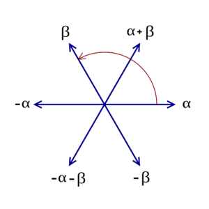
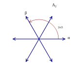
As a first example, consider the six vectors in 2-dimensional Euclidean space, R2, as shown in the image at the right; call them roots. These vectors span the whole space. If you consider the line perpendicular to any root, say β, then the reflection of R2 in that line sends any other root, say α, to another root. Moreover, the root to which it is sent equals α+ n β , where n is an integer (in this case, n equals 1). These six vectors satisfy the following definition, and therefore they form a root system; this one is known as A2.
Definition
Let V be a finite-dimensional Euclidean vector space, with the standard Euclidean inner product denoted by . A root system in V is a finite set Φ of non-zero vectors (called roots) that satisfy the following conditions:[2][3]

- The roots span V.
- The only scalar multiples of a root x ∈ Φ that belong to Φ are x itself and –x.
- For every root x ∈ Φ, the set Φ is closed under reflection through the hyperplane perpendicular to x.
- (Integrality) If x and y are roots in Φ, then the projection of y onto the line through x is a half-integral multiple of x.
An equivalent way of writing conditions 3 and 4 is as follows:
- For any two roots x and y, the set Φ contains the element
- For any two roots x and y, the number is an integer.


Some authors only include conditions 1–3 in the definition of a root system.[4] In this context, a root system that also satisfies the integrality condition is known as a crystallographic root system.[5] Other authors omit condition 2; then they call root systems satisfying condition 2 reduced.[6] In this article, all root systems are assumed to be reduced and crystallographic.
In view of property 3, the integrality condition is equivalent to stating that β and its reflection σα(β) differ by an integer multiple of α. Note that the operator

defined by property 4 is not an inner product. It is not necessarily symmetric and is linear only in the first argument.
 |
 |
| Root system |
Root system |
 |
 |
| Root system |
Root system |
 |
 |
| Root system |
Root system |


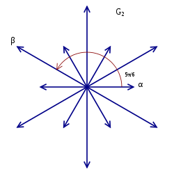
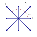
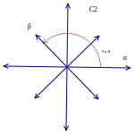
The rank of a root system Φ is the dimension of V. Two root systems may be combined by regarding the Euclidean spaces they span as mutually orthogonal subspaces of a common Euclidean space. A root system which does not arise from such a combination, such as the systems A2, B2, and G2 pictured to the right, is said to be irreducible.
Two root systems (E1, Φ1) and (E2, Φ2) are called isomorphic if there is an invertible linear transformation E1 → E2 which sends Φ1 to Φ2 such that for each pair of roots, the number is preserved.[7]

The group of isometries of V generated by reflections through hyperplanes associated to the roots of Φ is called the Weyl group of Φ. As it acts faithfully on the finite set Φ, the Weyl group is always finite.
The root lattice of a root system Φ is the Z-submodule of V generated by Φ. It is a lattice in V.
Rank two examples
There is only one root system of rank 1, consisting of two nonzero vectors . This root system is called .


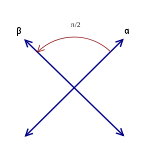
In rank 2 there are four possibilities, corresponding to , where .[8] Note that a root system is not determined by the lattice that it generates: and both generate a square lattice while and generate a hexagonal lattice, only two of the five possible types of lattices in two dimensions.


Whenever Φ is a root system in V, and U is a subspace of V spanned by Ψ = Φ ∩ U, then Ψ is a root system in U. Thus, the exhaustive list of four root systems of rank 2 shows the geometric possibilities for any two roots chosen from a root system of arbitrary rank. In particular, two such roots must meet at an angle of 0, 30, 45, 60, 90, 120, 135, 150, or 180 degrees.
History
The concept of a root system was originally introduced by Wilhelm Killing around 1889 (in German, Wurzelsystem[9]).[10] He used them in his attempt to classify all simple Lie algebras over the field of complex numbers. Killing originally made a mistake in the classification, listing two exceptional rank 4 root systems, when in fact there is only one, now known as F4. Cartan later corrected this mistake, by showing Killing's two root systems were isomorphic.[11]
Killing investigated the structure of a Lie algebra , by considering (what is now called) a Cartan subalgebra . Then he studied the roots of the characteristic polynomial , where . Here a root is considered as a function of , or indeed as an element of the dual vector space . This set of roots form a root system inside , as defined above, where the inner product is the Killing form.[12]


Elementary consequences of the root system axioms


Modulo reflection, for a given α there are only 5 nontrivial possibilities for β, and 3 possible angles between α and β in a set of simple roots. Subscript letters correspond to the series of root systems for which the given β can serve as the first root and α as the second root (or in F4 as the middle 2 roots).
The cosine of the angle between two roots is constrained to be a half-integral multiple of a square root of an integer. This is because and are both integers, by assumption, and

Since , the only possible values for are and , corresponding to angles of 90°, 60° or 120°, 45° or 135°, 30° or 150°, and 0° or 180°. Condition 2 says that no scalar multiples of α other than 1 and -1 can be roots, so 0 or 180°, which would correspond to 2α or −2α, are out.
![2\cos(\theta )\in [-2,2]](../I/m/9a5c767297a7512c69089c0b49082c5623727b25.svg)


Positive roots and simple roots
Given a root system Φ we can always choose (in many ways) a set of positive roots. This is a subset of Φ such that

- For each root exactly one of the roots , – is contained in .
- For any two distinct such that is a root, .


If a set of positive roots is chosen, elements of are called negative roots.

An element of is called a simple root if it cannot be written as the sum of two elements of . The set of simple roots is a basis of with the property that every vector in is a linear combination of elements of with all coefficients non-negative, or all coefficients non-positive.[13] For each choice of positive roots, the corresponding set of simple roots is the unique set of roots such that the positive roots are exactly those that can be expressed as a combination of them with non-negative coefficients, and such that these combinations are unique.


The root poset

The set of positive roots is naturally ordered by saying that if and only if is a nonnegative linear combination of simple roots. This poset is graded by , and has many remarkable combinatorial properties, one of them being that one can determine the degrees of the fundamental invariants of the corresponding Weyl group from this poset.[14] The Hasse graph is a visualization of the ordering of the root poset.


Dual root system and coroots
If Φ is a root system in V, the coroot α∨ of a root α is defined by

The set of coroots also forms a root system Φ∨ in V, called the dual root system (or sometimes inverse root system). By definition, α∨ ∨ = α, so that Φ is the dual root system of Φ∨. The lattice in V spanned by Φ∨ is called the coroot lattice. Both Φ and Φ∨ have the same Weyl group W and, for s in W,

If Δ is a set of simple roots for Φ, then Δ∨ is a set of simple roots for Φ∨.[15]
Classification of root systems by Dynkin diagrams
A root system is irreducible if it can not be partitioned into the union of two proper subsets , such that for all and .


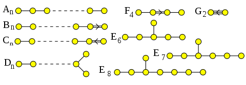
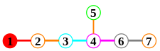
Irreducible root systems correspond to certain graphs, the Dynkin diagrams named after Eugene Dynkin. The classification of these graphs is a simple matter of combinatorics, and induces a classification of irreducible root systems.
Given a root system, select a set Δ of simple roots as in the preceding section. The vertices of the associated Dynkin diagram correspond to vectors in Δ. An edge is drawn between each non-orthogonal pair of vectors; it is an undirected single edge if they make an angle of radians, a directed double edge if they make an angle of radians, and a directed triple edge if they make an angle of radians. The term "directed edge" means that double and triple edges are marked with an angle sign pointing toward the shorter vector.


Although a given root system has more than one possible set of simple roots, the Weyl group acts transitively on such choices.[16] Consequently, the Dynkin diagram is independent of the choice of simple roots; it is determined by the root system itself. Conversely, given two root systems with the same Dynkin diagram, one can match up roots, starting with the roots in the base, and show that the systems are in fact the same.
Thus the problem of classifying root systems reduces to the problem of classifying possible Dynkin diagrams. Root systems are irreducible if and only if their Dynkin diagrams are connected. Dynkin diagrams encode the inner product on E in terms of the basis Δ, and the condition that this inner product must be positive definite turns out to be all that is needed to get the desired classification.
The actual connected diagrams are as follows. The subscripts indicate the number of vertices in the diagram (and hence the rank of the corresponding irreducible root system).
Properties of the irreducible root systems
| I | D | ||||
|---|---|---|---|---|---|
| An (n ≥ 1) | n(n + 1) | n + 1 | (n + 1)! | ||
| Bn (n ≥ 2) | 2n2 | 2n | 2 | 2 | 2n n! |
| Cn (n ≥ 3) | 2n2 | 2n(n − 1) | 2n−1 | 2 | 2n n! |
| Dn (n ≥ 4) | 2n(n − 1) | 4 | 2n − 1 n! | ||
| E6 | 72 | 3 | 51840 | ||
| E7 | 126 | 2 | 2903040 | ||
| E8 | 240 | 1 | 696729600 | ||
| F4 | 48 | 24 | 4 | 1 | 1152 |
| G2 | 12 | 6 | 3 | 1 | 12 |


Irreducible root systems are named according to their corresponding connected Dynkin diagrams. There are four infinite families (An, Bn, Cn, and Dn, called the classical root systems) and five exceptional cases (the exceptional root systems).[17] The subscript indicates the rank of the root system.
In an irreducible root system there can be at most two values for the length (α, α)1/2, corresponding to short and long roots. If all roots have the same length they are taken to be long by definition and the root system is said to be simply laced; this occurs in the cases A, D and E. Any two roots of the same length lie in the same orbit of the Weyl group. In the non-simply laced cases B, C, G and F, the root lattice is spanned by the short roots and the long roots span a sublattice, invariant under the Weyl group, equal to r2/2 times the coroot lattice, where r is the length of a long root.
In the adjacent table, |Φ<| denotes the number of short roots, I denotes the index in the root lattice of the sublattice generated by long roots, D denotes the determinant of the Cartan matrix, and |W| denotes the order of the Weyl group.
Explicit construction of the irreducible root systems
An
| e1 | e2 | e3 | e4 | |
|---|---|---|---|---|
| α1 | 1 | −1 | 0 | 0 |
| α2 | 0 | 1 | −1 | 0 |
| α3 | 0 | 0 | 1 | −1 |
Let V be the subspace of Rn+1 for which the coordinates sum to 0, and let Φ be the set of vectors in V of length √2 and which are integer vectors, i.e. have integer coordinates in Rn+1. Such a vector must have all but two coordinates equal to 0, one coordinate equal to 1, and one equal to –1, so there are n2 + n roots in all. One choice of simple roots expressed in the standard basis is: αi = ei – ei+1, for 1 ≤ i ≤ n.
The reflection σi through the hyperplane perpendicular to αi is the same as permutation of the adjacent i-th and (i + 1)-th coordinates. Such transpositions generate the full permutation group. For adjacent simple roots, σi(αi+1) = αi+1 + αi = σi+1(αi) = αi + αi+1, that is, reflection is equivalent to adding a multiple of 1; but reflection of a simple root perpendicular to a nonadjacent simple root leaves it unchanged, differing by a multiple of 0.
The An root lattice - that is, the lattice generated by the An roots - is most easily described as the set of integer vectors in Rn+1 whose components sum to zero.
The A3 root lattice is known to crystallographers as the face-centered cubic (fcc) (or cubic close packed) lattice.[18]

The A3 root system (as well as the other rank-three root systems) may be modeled in the Zometool Construction set.[19]
Bn
| 1 | -1 | 0 | 0 |
| 0 | 1 | -1 | 0 |
| 0 | 0 | 1 | -1 |
| 0 | 0 | 0 | 1 |
Let V = Rn, and let Φ consist of all integer vectors in V of length 1 or √2. The total number of roots is 2n2. One choice of simple roots is: αi = ei – ei+1, for 1 ≤ i ≤ n – 1 (the above choice of simple roots for An-1), and the shorter root αn = en.
The reflection σn through the hyperplane perpendicular to the short root αn is of course simply negation of the nth coordinate. For the long simple root αn-1, σn-1(αn) = αn + αn-1, but for reflection perpendicular to the short root, σn(αn-1) = αn-1 + 2αn, a difference by a multiple of 2 instead of 1.
The Bn root lattice - that is, the lattice generated by the Bn roots - consists of all integer vectors.
B1 is isomorphic to A1 via scaling by √2, and is therefore not a distinct root system.
Cn
| 1 | -1 | 0 | 0 |
| 0 | 1 | -1 | 0 |
| 0 | 0 | 1 | -1 |
| 0 | 0 | 0 | 2 |
Let V = Rn, and let Φ consist of all integer vectors in V of length √2 together with all vectors of the form 2λ, where λ is an integer vector of length 1. The total number of roots is 2n2. One choice of simple roots is: αi = ei – ei+1, for 1 ≤ i ≤ n – 1 (the above choice of simple roots for An-1), and the longer root αn = 2en. The reflection σn(αn-1) = αn-1 + αn, but σn-1(αn) = αn + 2αn-1.
The Cn root lattice - that is, the lattice generated by the Cn roots - consists of all integer vectors whose components sum to an even integer.
C2 is isomorphic to B2 via scaling by √2 and a 45 degree rotation, and is therefore not a distinct root system.
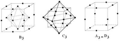
Root system B3, C3, and A3=D3 as points within a cube and octahedron
Dn
| 1 | -1 | 0 | 0 |
| 0 | 1 | -1 | 0 |
| 0 | 0 | 1 | -1 |
| 0 | 0 | 1 | 1 |
 | |||
Let V = Rn, and let Φ consist of all integer vectors in V of length √2. The total number of roots is 2n(n – 1). One choice of simple roots is: αi = ei – ei+1, for 1 ≤ i < n (the above choice of simple roots for An-1) plus αn = en + en-1.
Reflection through the hyperplane perpendicular to αn is the same as transposing and negating the adjacent n-th and (n – 1)-th coordinates. Any simple root and its reflection perpendicular to another simple root differ by a multiple of 0 or 1 of the second root, not by any greater multiple.
The Dn root lattice - that is, the lattice generated by the Dn roots - consists of all integer vectors whose components sum to an even integer. This is the same as the Cn root lattice.
D3 coincides with A3, and is therefore not a distinct root system.
D4 has additional symmetry called triality.
E6, E7, E8
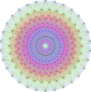
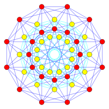
 72 vertices of 122 represent the root vectors of E6 (Green nodes are doubled in this E6 Coxeter plane projection) |
 126 vertices of 231 represent the root vectors of E7 |
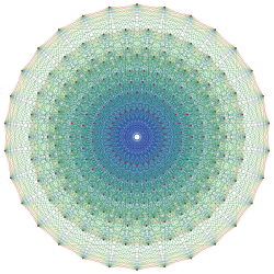 240 vertices of 421 represent the root vectors of E8 |
 |
 |
 |
- The E8 root system is any set of vectors in R8 that is congruent to the following set:
- D8 ∪ { ½( ∑i=18 εiei) : εi = ±1, ε1•••ε8 = +1}.
The root system has 240 roots. The set just listed is the set of vectors of length √2 in the E8 root lattice, also known simply as the E8 lattice or Γ8. This is the set of points in R8 such that:
- all the coordinates are integers or all the coordinates are half-integers (a mixture of integers and half-integers is not allowed), and
- the sum of the eight coordinates is an even integer.
Thus,
- E8 = {α ∈ Z8 ∪ (Z+½)8 : |α|2 = ∑αi2 = 2, ∑αi ∈ 2Z}.
- The root system E7 is the set of vectors in E8 that are perpendicular to a fixed root in E8. The root system E7 has 126 roots.
- The root system E6 is not the set of vectors in E7 that are perpendicular to a fixed root in E7, indeed, one obtains D6 that way. However, E6 is the subsystem of E8 perpendicular to two suitably chosen roots of E8. The root system E6 has 72 roots.
| 1 | -1 | 0 | 0 | 0 | 0 | 0 | 0 |
| 0 | 1 | -1 | 0 | 0 | 0 | 0 | 0 |
| 0 | 0 | 1 | -1 | 0 | 0 | 0 | 0 |
| 0 | 0 | 0 | 1 | -1 | 0 | 0 | 0 |
| 0 | 0 | 0 | 0 | 1 | -1 | 0 | 0 |
| 0 | 0 | 0 | 0 | 0 | 1 | -1 | 0 |
| 0 | 0 | 0 | 0 | 0 | 1 | 1 | 0 |
| -½ | -½ | -½ | -½ | -½ | -½ | -½ | -½ |
An alternative description of the E8 lattice which is sometimes convenient is as the set Γ'8 of all points in R8 such that
- all the coordinates are integers and the sum of the coordinates is even, or
- all the coordinates are half-integers and the sum of the coordinates is odd.
The lattices Γ8 and Γ'8 are isomorphic; one may pass from one to the other by changing the signs of any odd number of coordinates. The lattice Γ8 is sometimes called the even coordinate system for E8 while the lattice Γ'8 is called the odd coordinate system.
One choice of simple roots for E8 in the even coordinate system with rows ordered by node order in the alternate (non-canonical) Dynkin diagrams (above) is:
- αi = ei – ei+1, for 1 ≤ i ≤ 6, and
- α7 = e7 + e6
(the above choice of simple roots for D7) along with
- α8 = β0 = = (-½,-½,-½,-½,-½,-½,-½,-½).

| 1 | -1 | 0 | 0 | 0 | 0 | 0 | 0 |
| 0 | 1 | -1 | 0 | 0 | 0 | 0 | 0 |
| 0 | 0 | 1 | -1 | 0 | 0 | 0 | 0 |
| 0 | 0 | 0 | 1 | -1 | 0 | 0 | 0 |
| 0 | 0 | 0 | 0 | 1 | -1 | 0 | 0 |
| 0 | 0 | 0 | 0 | 0 | 1 | -1 | 0 |
| 0 | 0 | 0 | 0 | 0 | 0 | 1 | -1 |
| -½ | -½ | -½ | -½ | -½ | ½ | ½ | ½ |
One choice of simple roots for E8 in the odd coordinate system with rows ordered by node order in alternate (non-canonical) Dynkin diagrams (above) is:
- αi = ei – ei+1, for 1 ≤ i ≤ 7
(the above choice of simple roots for A7) along with
- α8 = β5, where
- βj = .

(Using β3 would give an isomorphic result. Using β1,7 or β2,6 would simply give A8 or D8. As for β4, its coordinates sum to 0, and the same is true for α1...7, so they span only the 7-dimensional subspace for which the coordinates sum to 0; in fact –2β4 has coordinates (1,2,3,4,3,2,1) in the basis (αi).)
Since perpendicularity to α1 means that the first two coordinates are equal, E7 is then the subset of E8 where the first two coordinates are equal, and similarly E6 is the subset of E8 where the first three coordinates are equal. This facilitates explicit definitions of E7 and E6 as:
- E7 = {α ∈ Z7 ∪ (Z+½)7 : ∑αi2 + α12 = 2, ∑αi + α1 ∈ 2Z},
- E6 = {α ∈ Z6 ∪ (Z+½)6 : ∑αi2 + 2α12 = 2, ∑αi + 2α1 ∈ 2Z}
Note that deleting α1 and then α2 gives sets of simple roots for E7 and E6. However, these sets of simple roots are in different E7 and E6 subspaces of E8 than the ones written above, since they are not orthogonal to α1 or α2.
F4
| 1 | -1 | 0 | 0 |
| 0 | 1 | -1 | 0 |
| 0 | 0 | 1 | 0 |
| -½ | -½ | -½ | -½ |
For F4, let V = R4, and let Φ denote the set of vectors α of length 1 or √2 such that the coordinates of 2α are all integers and are either all even or all odd. There are 48 roots in this system. One choice of simple roots is: the choice of simple roots given above for B3, plus α4 = – .

The F4 root lattice - that is, the lattice generated by the F4 root system - is the set of points in R4 such that either all the coordinates are integers or all the coordinates are half-integers (a mixture of integers and half-integers is not allowed). This lattice is isomorphic to the lattice of Hurwitz quaternions.
G2
| 1 | -1 | 0 |
| -1 | 2 | -1 |
The root system G2 has 12 roots, which form the vertices of a hexagram. See the picture above.
One choice of simple roots is: (α1, β = α2 – α1) where αi = ei – ei+1 for i = 1, 2 is the above choice of simple roots for A2.
The G2 root lattice - that is, the lattice generated by the G2 roots - is the same as the A2 root lattice.
Root systems and Lie theory
Irreducible root systems classify a number of related objects in Lie theory, notably the
- simple Lie groups (see the list of simple Lie groups), including the
- simple complex Lie groups;
- their associated simple complex Lie algebras; and
- simply connected complex Lie groups which are simple modulo centers.
In each case, the roots are non-zero weights of the adjoint representation.
In the case of a simply connected simple compact Lie group G with maximal torus T, the root lattice can naturally be identified with Hom(T, T) and the coroot lattice with Hom(T, T), where T is the circle group; see Adams (1983).
For connections between the exceptional root systems and their Lie groups and Lie algebras see E8, E7, E6, F4, and G2.
See also
- ADE classification
- Affine root system
- Coxeter–Dynkin diagram
- Coxeter group
- Coxeter matrix
- Dynkin diagram
- root datum
- Root system of a semi-simple Lie algebra
- Weyl group
Notes
- ↑ "Graphs with least eigenvalue −2; a historical survey and recent developments in maximal exceptional graphs". Linear Algebra and its Applications. 356: 189–210. doi:10.1016/S0024-3795(02)00377-4.
- ↑ Bourbaki, Ch.VI, Section 1
- ↑ Humphreys (1972), p.42
- ↑ Humphreys (1992), p.6
- ↑ Humphreys (1992), p.39
- ↑ Humphreys (1992), p.41
- ↑ Humphreys (1972), p.43
- ↑ Hall 2015 Proposition 8.8
- ↑ Killing (1889)
- ↑ Bourbaki (1998), p.270
- ↑ Coleman, p.34
- ↑ Bourbaki (1998), p.270
- ↑ Hall 2015 Theorem 8.16
- ↑ Humphreys (1992), Theorem 3.20
- ↑ Hall 2015 Proposition 8.18
- ↑ This follows from Hall 2015 Proposition 8.23
- ↑ Hall, Brian C. (2003), Lie Groups, Lie Algebras, and Representations: An Elementary Introduction, Springer, ISBN 0-387-40122-9.
- ↑ Conway, John Horton; Sloane, Neil James Alexander; & Bannai, Eiichi. Sphere packings, lattices, and groups. Springer, 1999, Section 6.3.
- ↑ Hall 2015 Section 8.9
References
- Adams, J.F. (1983), Lectures on Lie groups, University of Chicago Press, ISBN 0-226-00530-5
- Bourbaki, Nicolas (2002), Lie groups and Lie algebras, Chapters 4–6 (translated from the 1968 French original by Andrew Pressley), Elements of Mathematics, Springer-Verlag, ISBN 3-540-42650-7. The classic reference for root systems.
- Bourbaki, Nicolas (1998). Elements of the History of Mathematics. Springer. ISBN 3540647678.
- A.J. Coleman (Summer 1989), "The greatest mathematical paper of all time", The Mathematical Intelligencer, 11 (3): 29–38, doi:10.1007/bf03025189
- Hall, Brian C. (2015), Lie groups, Lie algebras, and representations: An elementary introduction, Graduate Texts in Mathematics, 222 (2nd ed.), Springer
- Humphreys, James (1992). Reflection Groups and Coxeter Groups. Cambridge University Press. ISBN 0521436133.
- Humphreys, James (1972). Introduction to Lie algebras and Representation Theory. Springer. ISBN 0387900535.
- Killing, Die Zusammensetzung der stetigen endlichen Transformationsgruppen Mathematische Annalen, Part 1: Volume 31, Number 2 June 1888, Pages 252-290 doi:10.1007/BF01211904; Part 2: Volume 33, Number 1 March 1888, Pages 1–48 doi:10.1007/BF01444109; Part3: Volume 34, Number 1 March 1889, Pages 57–122 doi:10.1007/BF01446792; Part 4: Volume 36, Number 2 June 1890,Pages 161-189 doi:10.1007/BF01207837
- Kac, Victor G. (1994), Infinite dimensional Lie algebras.
- Springer, T.A. (1998). Linear Algebraic Groups, Second Edition. Birkhäuser. ISBN 0817640215.
Further reading
- Dynkin, E. B. The structure of semi-simple algebras. (Russian) Uspehi Matem. Nauk (N.S.) 2, (1947). no. 4(20), 59–127.
External links
| Wikimedia Commons has media related to Root systems. |