SNV calling from NGS data
SNV calling from NGS data refers to a range of methods for identifying the existence of single nucleotide variants (SNVs) from the results of next generation sequencing (NGS) experiments. These are computational techniques, and are in contrast to special experimental methods based on known population-wide single nucleotide polymorphisms (see SNP genotyping). Due to the increasing abundance of NGS data, these techniques are becoming increasingly popular for performing SNP genotyping, with a wide variety of algorithms designed for specific experimental designs and applications.[1] In addition to the usual application domain of SNP genotyping, these techniques have been successfully adapted to identify rare SNPs within a population,[2] as well as detecting somatic SNVs within an individual using multiple tissue samples.[3]
Methods for detecting germline variants
Most NGS based methods for SNV detection are designed to detect germline variations in the individual's genome. These are the mutations that an individual biologically inherits from their parents, and are the usual type of variants searched for when performing such analysis (except for certain specific applications where somatic mutations are sought). Very often, the searched for variants occur with some (possibly rare) frequency, throughout the population, in which case they may be referred to as single nucleotide polymorphisms (SNPs). Technically the term SNP only refers to these kinds of variations, however in practice they are often used synonymously with SNV in the literature on variant calling. In addition, since the detection of germline SNVs requires determining the individual's genotype at each locus, the phrase "SNP genotyping" may also be used to refer to this process. However this phrase may also refer to wet-lab experimental procedures for classifying genotypes at a set of known SNP locations.
The usual process of such techniques are based around:[1]
- Filtering the set of NGS reads to remove sources of error/bias
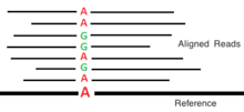
- Aligning the reads to a reference genome
- Using an algorithm, either based on a statistical model or some heuristics, to predict the likelihood of variation at each locus, based on the quality scores and allele counts of the aligned reads at that locus
- Filtering the predicted results, often based on metrics relevant to the application
- SNP annotation to predict the functional effect of each variation.
The usual output of these procedures is a VCF file.
Probabilistic methods
In an ideal error free world with high read coverage, the task of variant calling from the results of a NGS data alignment would be simple; at each locus (position on the genome) the number of occurrences of each distinct nucleotide among the reads aligned at that position can be counted, and the true genotype would be obvious; either AA if all nucleotides match allele A, BB if they match allele B, or AB if there is a mixture. However, when working with real NGS data this sort of naive approach is not used, as it cannot account for the noise in the input data.[4] The nucleotide counts used for base calling contain errors and bias, both due do the sequenced reads themselves, and the alignment process. This issue can be mitigated to some extent by sequencing to a greater depth of read coverage, however this is often expensive, and many practical studies require making inferences on low coverage data.[1]
Probabilistic methods aim to overcome the above issue, by producing robust estimates of the probabilities of each of the possible genotypes, taking into account noise, as well as other available prior information that can be used to improve estimates. A genotype can then be predicted based on these probabilities, often according to the MAP estimate.
Probabilistic methods for variant calling are based on Bayes' Theorem. In the context of variant calling, Bayes' Theorem defines the probability of each genotype being the true genotype given the observed data, in terms of the prior probabilities of each possible genotype, and the probability distribution of the data given each possible genotype. The formula is:
![{\begin{aligned}P(G|D)&={\frac {P(D|G)P(G)}{P(D)}}\\[8pt]&={\frac {P(D|G)\,P(G)}{\sum \limits _{{i=1}}^{{n}}P(D|G_{i})\,P(G_{i})}}\\[8pt]\end{aligned}}](../I/m/3df7037b93615fffbdd732697cd7730974f0e8bc.svg)
In the above equation:
- refers to the observed data; that is, the aligned reads
- is the genotype whose probability is being calculated
- refers to the ith possible genotype, out of n possibilities


Given the above framework, different software solutions for detecting SNVs vary based on how they calculate the prior probabilities , the error model used to model the probabilities , and the partitioning of the overall genotypes into separate sub-genotypes, whose probabilities can be individually estimated in this framework.[5]


Prior genotype probability estimation
The calculation of prior probabilities depends on available data from the genome being studied, and the type of analysis being performed. For studies where good reference data containing frequencies of known mutations is available (for example, in studying human genome data), these known frequencies of genotypes in the population can be used to estimate priors. Given population wide allele frequencies, prior genotype probabilities can be calculated at each locus according to the Hardy Weinberg Equilibrium.[6] In the absence of such data, constant priors can be used, independent of the locus. These can be set using heuristically chosen values, possibly informed by the kind of variations being sought by the study. Alternatively, supervised machine-learning procedures have been investigated that seek to learn optimal prior values for individuals in a sample, using supplied NGS data from these individuals.[4]
Error models for data observations
The error model used in creating a probabilistic method for variant calling is the basis for calculating the term used in Bayes' theorem. If the data was assumed to be error free, then the distribution of observed nucleotide counts at each locus would follow a Binomial Distribution, with 100% of nucleotides matching the A or B allele respectively in the AA and BB cases, and a 50% chance of each nucleotide matching either A or B in the AB case. However, in presence of noise in the read data this assumption is violated, and the values need to account for the possibility that erroneous nucleotides are present in the aligned reads at each locus.
A simple error model is to introduce a small error to the data probability term in the homozygous cases, allowing a small constant probability that nucleotides which don't match the A allele are observed in the AA case, and respectively a small constant probability that nucleotides not matching the B allele are observed in the BB case. However more sophisticated procedures are available which attempt to more realistically replicate the actual error patterns observed in real data in calculating the conditional data probabilities. For instance, estimations of read quality (measured as Phred quality scores) have been incorporated in these calculations, taking into account the expected error rate in each individual read at a locus.[7] Another technique that has successfully been incorporated into error models is base quality recalibration, where separate error rates are calculated - based on prior known information about error patterns - for each possible nucleotide substitution. Research shows that each possible nucleotide substitution is not equally likely to show up as an error in sequencing data, and so base quality recalibration has been applied to improve error probability estimates.[6]
Partitioning of the genotype
In the above discussion, it has been assumed that the genotype probabilities at each locus are calculated independently; that is, the entire genotype is partitioned into independent genotypes at each locus, whose probabilities are calculated independently. However, due to linkage disequilibrium the genotypes of nearby loci are in general not independent. As a result, partitioning the overall genotype instead into a sequence of overlapping haplotypes allows these correlations to be modelled, resulting in more precise probability estimates through the incorporation of population-wide haplotype frequencies in the prior. The use of haplotypes to improve variant detection accuracy has been applied successfully, for instance in the 1000 Genomes Project.[8]
Heuristic based algorithms
As an alternative to probabilistic methods, heuristic methods exist for performing variant calling on NGS data. Instead of modelling the distribution of the observed data and using Bayesian statistics to calculate genotype probabilities, variant calls are made based on a variety of heuristic factors, such as minimum allele counts, read quality cut-offs, bounds on read depth, etc. Although they have been relatively unpopular in practice in comparison to probabilistic methods, in practice due to their use of bounds and cut-offs they can be robust to outlying data that violate the assumptions of probabilistic models.[9]
Reference genome used for alignment
An important part of the design of variant calling methods using NGS data is the DNA sequence used as a reference to align the NGS reads to. In human genetics studies, high quality references are available, from sources such as the HapMap project,[10] which can substantially improve the accuracy of the variant calls made by variant calling algorithms. As a bonus, such references can be a source of prior genotype probabilities for Bayesian-based analysis. However, in the absence of such a high quality reference, experimentally obtained reads can first be assembled in order to create a reference sequence for alignment.[1]
Pre-processing and filtering of results
Various methods exist for filtering data in variant calling experiments, in order to remove sources of error/bias. This can involve the removal of suspicious reads before performing alignment and/or filtering of the list of variants returned by the variant calling algorithm.
Depending on the sequencing platform used, various biases may exist within the set of sequenced reads. For instance, strand bias can occur, where there is a highly unequal distribution of forward vs reverse directions in the reads aligned in some neighborhood. Additionally, there may occur an unusually high duplication of some reads (for instance due to bias in PCR). Such biases can result in dubious variant calls - for instance if a fragment containing a PCR error at some locus is over amplified due to PCR bias, that locus will have a high count of the false allele, and may be called as a SNV - and so analysis pipelines frequently filter calls based on these biases.[1]
Methods for detecting somatic variants
In addition to methods that align reads from individual sample(s) to a reference genome in order to detect germline genetic variants, reads from multiple tissue samples within a single individual can be aligned and compared in order to detect somatic variants. These variants correspond to mutations that have occurred de novo within groups of somatic cells within an individual (that is, they are not present within the individual's germline cells). This form of analysis has been frequently applied to the study of cancer, where many studies are designed around investigating the profile of somatic mutations within cancerous tissues. Such investigations have resulted in diagnostic tools that have seen clinical application, and are used to improve scientific understanding of the disease, for instance by the discovery of new cancer-related genes, identification of involved gene regulatory networks and metabolic pathways, and by informing models of how tumors grow and evolve.[11]
Recent developments
Until recently, software tools for carrying out this form of analysis have been heavily underdeveloped, and were based on the same algorithms used to detect germline variations. Such procedures are not optimized for this task, because they do not adequately model the statistical correlation between the genotypes present in multiple tissue samples from the same individual.[3]
More recent investigations have resulted in the development of software tools especially optimized for the detection of somatic mutations from multiple tissue samples. Probabilistic techniques have been developed that pool allele counts from all tissue samples at each locus, and using statistical models for the likelihoods of joint-genotypes for all the tissues, and the distribution of allele counts given the genotype, are able to calculate relatively robust probabilities of somatic mutations at each locus using all available data.[3][12] In addition there has recently been some investigation in machine learning based techniques for performing this analysis.[13]
List of available software
- SOAPsnp
- realSFS
- SAMtools
- GATK
- Beagle
- IMPUTE2
- MaCH
- SNVmix
- VarScan
- Somaticsniper
- JointSNVMix
- Big Data Genomics: Avocado
- NGSEP
- VarDict
- Reveel
References
- 1 2 3 4 5 Nielsen, Rasmus and Paul, Joshua S and Albrechtsen, Anders and Song, Yun S (2011). "Genotype and SNP calling from next-generation sequencing data". Nature Reviews Genetics. Nature Publishing Group. 12 (6): 443–451. doi:10.1038/nrg2986.
- ↑ Bansal, Vikas (2010). "A statistical method for the detection of variants from next-generation resequencing of DNA pools". Bioinformatics. Oxford University Press. 26 (12): i318–i324. doi:10.1093/bioinformatics/btq214.
- 1 2 3 Roth, Andrew and Ding, Jiarui and Morin, Ryan and Crisan, Anamaria and Ha, Gavin and Giuliany, Ryan and Bashashati, Ali and Hirst, Martin and Turashvili, Gulisa and Oloumi, Arusha; et al. (2012). "JointSNVMix: a probabilistic model for accurate detection of[somatic mutations in normal/tumour paired next-generation sequencing data". Bioinformatics. Oxford University Press. 28 (7): 907–913. doi:10.1093/bioinformatics/bts053.
- 1 2 Martin, Eden R and Kinnamon, DD and Schmidt, Michael A and Powell, EH and Zuchner, S and Morris, RW (2010). "SeqEM: an adaptive genotype-calling approach for next-generation sequencing studies". Bioinformatics. Oxford University Press. 26 (22): 2803–2810. doi:10.1093/bioinformatics/btq526.
- ↑ You, Na and Murillo, Gabriel and Su, Xiaoquan and Zeng, Xiaowei and Xu, Jian and Ning, Kang and Zhang, Shoudong and Zhu, Jiankang and Cui, Xinping (2012). "SNP calling using genotype model selection on high-throughput sequencing data". Bioinformatics. Oxford University Press. 28 (5): 643–650. doi:10.1093/bioinformatics/bts001.
- 1 2 Li, Ruiqiang and Li, Yingrui and Fang, Xiaodong and Yang, Huanming and Wang, Jian and Kristiansen, Karsten and Wang, Jun (2009). "SNP detection for massively parallel whole-genome resequencing". Genome Research. Cold Spring Harbor Lab. 19 (6): 1124–1132. doi:10.1101/gr.088013.108.
- ↑ Li, Heng and Ruan, Jue and Durbin, Richard (2008). "Mapping short DNA sequencing reads and calling variants using mapping quality scores". Genome Research. Cold Spring Harbor Lab. 18 (11): 1851–1858. doi:10.1101/gr.078212.108. PMC 2577856
 . PMID 18714091.
 - ↑ Abecasis, GR and Altshuler, David and Auton, A and Brooks, LD and Durbin, RM and Gibbs, Richard A and Hurles, Matt E and McVean, Gil A and Bentley, DR and Chakravarti, A; et al. (2010). "A map of human genome variation from population-scale sequencing.". Nature. 467 (7319): 1061–1073. doi:10.1038/nature09534. PMC 3042601. PMID 20981092.
- ↑ Koboldt, Daniel C and Zhang, Qunyuan and Larson, David E and Shen, Dong and McLellan, Michael D and Lin, Ling and Miller, Christopher A and Mardis, Elaine R and Ding, Li and Wilson, Richard K (2012). "VarScan 2: somatic mutation and copy number alteration discovery in cancer by exome sequencing". Genome Research. Cold Spring Harbor Lab. 22 (3): 568–576. doi:10.1101/gr.129684.111. PMC 3290792. PMID 22300766.
- ↑ Gibbs, Richard A and Belmont, John W and Hardenbol, Paul and Willis, Thomas D and Yu, Fuli and Yang, Huanming and Ch'ang, Lan-Yang and Huang, Wei and Liu, Bin and Shen, Yan; et al. (2003). "The international HapMap project". Nature. Nature Publishing Group. 426 (6968): 789–796. doi:10.1038/nature02168. PMID 14685227.
- ↑ Shyr, Derek; Liu, Qi; et al. (2013). "Next generation sequencing in cancer research and clinical application". Biological procedures online. 15 (4).
- ↑ Larson, David E and Harris, Christopher C and Chen, Ken and Koboldt, Daniel C and Abbott, Travis E and Dooling, David J and Ley, Timothy J and Mardis, Elaine R and Wilson, Richard K and Ding, Li (2012). "SomaticSniper: identification of somatic point mutations in whole genome sequencing data". Bioinformatics. Oxford University Press. 28 (3): 311–317. doi:10.1093/bioinformatics/btr665.
- ↑ Ding, Jiarui and Bashashati, Ali and Roth, Andrew and Oloumi, Arusha and Tse, Kane and Zeng, Thomas and Haffari, Gholamreza and Hirst, Martin and Marra, Marco A and Condon, Anne; et al. (2012). "Feature-based classifiers for somatic mutation detection in tumour--normal paired sequencing data". Bioinformatics. Oxford University Press. 28 (2): 167–175. doi:10.1093/bioinformatics/btr629.