Bollinger Bands
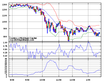
Bollinger Bands is a tool invented by John Bollinger in the 1980s as well as a term trademarked by him in 2011.[1] Having evolved from the concept of trading bands, Bollinger Bands and the related indicators %b and bandwidth can be used to measure the "highness" or "lowness" of the price relative to previous trades. Bollinger Bands are a volatility indicator similar to the Keltner channel.
Bollinger Bands consist of:
- an N-period moving average (MA)
- an upper band at K times an N-period standard deviation above the moving average (MA + Kσ)
- a lower band at K times an N-period standard deviation below the moving average (MA − Kσ)
Typical values for N and K are 20 and 2, respectively. The default choice for the average is a simple moving average, but other types of averages can be employed as needed. Exponential moving averages is a common second choice.[note 1] Usually the same period is used for both the middle band and the calculation of standard deviation.[note 2]
Purpose
The purpose of Bollinger Bands is to provide a relative definition of high and low. By definition, prices are high at the upper band and low at the lower band. This definition can aid in rigorous pattern recognition and is useful in comparing price action to the action of indicators to arrive at systematic trading decisions.[3]
Indicators derived from Bollinger Bands
In Spring, 2010, John Bollinger introduced three new indicators based on Bollinger Bands. They are BBImpulse, which measures price change as a function of the bands; percent bandwidth (%b), which normalizes the width of the bands over time; and bandwidth delta, which quantifies the changing width of the bands.
%b (pronounced "percent b") is derived from the formula for Stochastics and shows where price is in relation to the bands. %b equals 1 at the upper band and 0 at the lower band. Writing upperBB for the upper Bollinger Band, lowerBB for the lower Bollinger Band, and last for the last (price) value:
- %b = (last − lowerBB) / (upperBB − lowerBB)
Bandwidth tells how wide the Bollinger Bands are on a normalized basis. Writing the same symbols as before, and middleBB for the moving average, or middle Bollinger Band:
- Bandwidth = (upperBB − lowerBB) / middleBB
Using the default parameters of a 20-period look back and plus/minus two standard deviations, bandwidth is equal to four times the 20-period coefficient of variation.
Uses for %b include system building and pattern recognition. Uses for bandwidth include identification of opportunities arising from relative extremes in volatility and trend identification.
Interpretation
The use of Bollinger Bands varies widely among traders. Some traders buy when price touches the lower Bollinger Band and exit when price touches the moving average in the center of the bands. Other traders buy when price breaks above the upper Bollinger Band or sell when price falls below the lower Bollinger Band.[4] Moreover, the use of Bollinger Bands is not confined to stock traders; options traders, most notably implied volatility traders, often sell options when Bollinger Bands are historically far apart or buy options when the Bollinger Bands are historically close together, in both instances, expecting volatility to revert towards the average historical volatility level for the stock.
When the bands lie close together, a period of low volatility is indicated.[5] Conversely, as the bands expand, an increase in price action/market volatility is indicated.[5] When the bands have only a slight slope and track approximately parallel for an extended time, the price will generally be found to oscillate between the bands as though in a channel.
Traders are often inclined to use Bollinger Bands with other indicators to confirm price action. In particular, the use of oscillator-like Bollinger Bands will often be coupled with a non-oscillator indicator-like chart patterns or a trendline. If these indicators confirm the recommendation of the Bollinger Bands, the trader will have greater conviction that the bands are predicting correct price action in relation to market volatility.
Effectiveness
Various studies of the effectiveness of the Bollinger Band strategy have been performed with mixed results. In 2007 Lento et al. published an analysis using a variety of formats (different moving average timescales, and standard deviation ranges) and markets (e.g., Dow Jones and Forex).[6] Analysis of the trades, spanning a decade from 1995 onwards, found no evidence of consistent performance over the standard "buy and hold" approach. The authors did, however, find that a simple reversal of the strategy ("contrarian Bollinger Band") produced positive returns in a variety of markets.
Similar results were found in another study, which concluded that Bollinger Band trading strategies may be effective in the Chinese marketplace, stating: "Finally, we find significant positive returns on buy trades generated by the contrarian version of the moving-average crossover rule, the channel breakout rule, and the Bollinger Band trading rule, after accounting for transaction costs of 0.50 percent."[7] (By "the contrarian version", they mean buying when the conventional rule mandates selling, and vice versa.) A recent study examined the application of Bollinger Band trading strategies combined with the ADX for Equity Market indices with similar results.[8]
A paper from 2008 uses Bollinger Bands in forecasting the yield curve.[9]
Companies like Forbes suggest that the use of Bollinger Bands is a simple and often an effective strategy but stop-loss orders should be used to mitigate losses from market pressure.[10]
Statistical properties
Security price returns have no known statistical distribution, normal or otherwise; they are known to have fat tails, compared to a normal distribution.[11] The sample size typically used, 20, is too small for conclusions derived from statistical techniques like the central limit theorem to be reliable. Such techniques usually require the sample to be independent and identically distributed, which is not the case for a time series like security prices. Just the opposite is true; it is well recognized by practitioners that such price series are very commonly serially correlated—that is, each price will be closely related to its ancestor "most of the time". Adjusting for serial correlation is the purpose of moving standard deviations, which use deviations from the moving average, but the possibility remains of high order price autocorrelation not accounted for by simple differencing from the moving average.
For such reasons, it is incorrect to assume that the long-term percentage of the data that will be observed in the future outside the Bollinger Bands range will always be constrained to a certain amount. Instead of finding about 95% of the data inside the bands, as would be the expectation with the default parameters if the data were normally distributed, studies have found that only about 88% of security prices (85%-90%) remain within the bands.[12] For an individual security, one can always find factors for which certain percentages of data are contained by the factor defined bands for a certain period of time. Practitioners may also use related measures such as the Keltner channels, or the related Stoller average range channels, which base their band widths on different measures of price volatility, such as the difference between daily high and low prices, rather than on standard deviation.
Bollinger bands outside of finance
In a paper published in 2006 by the Society of Photo-Optical Engineers, "Novel method for patterned fabric inspection using Bollinger bands", Henry Y. T. Ngan and Grantham K. H. Pang present a method of using Bollinger bands to detect defects (anomalies) in patterned fabrics. From the abstract: "In this paper, the upper band and lower band of Bollinger Bands, which are sensitive to any subtle change in the input data, have been developed for use to indicate the defective areas in patterned fabric."[13]
The International Civil Aviation Organization is using Bollinger bands to measure the accident rate as a safety indicator to measure efficiency of global safety initiatives.[14] %b and bandwidth are also used in this analysis.
Notes
- ↑ When the average used in the calculation of Bollinger Bands is changed from a simple moving average to an exponential or weighted moving average, it must be changed for both the calculation of the middle band and the calculation of standard deviation.[2]
- ↑ Since Bollinger Bands use the population method of calculating standard deviation, the proper divisor for the sigma calculation is n, not n − 1.
References
- ↑ "Bollinger Bands – Trademark Details". Justia.com. 2011-12-20.
- ↑ Bollinger On Bollinger Bands – The Seminar, DVD I ISBN 978-0-9726111-0-7
- ↑ second paragraph, center column
- ↑ Technical Analysis: The Complete Resource for Financial Market Technicians by Charles D. Kirkpatrick and Julie R. Dahlquist Chapter 14
- 1 2 Baiynd, Anne-Marie (2011). The Trading Book: A Complete Solution to Mastering Technical Systems and Trading Psychology. McGraw-Hill. p. 272. ISBN 9780071766494. Retrieved 2013-04-30.
- ↑ Lento, C.; Gradojevic, N.; Wright, C. S. (2007). "Investment information content in Bollinger Bands?". Applied Financial Economics Letters. 3 (4): 263–267. doi:10.1080/17446540701206576. ISSN 1744-6546.
- ↑ Balsara, Nauzer J.; Chen, Gary; Zheng, Lin (2007). "The Chinese Stock Market: An Examination of the Random Walk Model and Technical Trading Rules". Quarterly Journal of Business and Economics. 46 (2): 43–63. JSTOR 40473435.
- ↑ Lim, Shawn; Hisarli, Tilman; Shi He, Ng (2014). "The Profitability of a Combined Signal Approach: Bollinger Bands and the ADX". International Federation of Technical Analysts Journal: 23–29.
- ↑ Rostan, Pierre; Théoret, Raymond; El moussadek, Abdeljalil (2008). "Forecasting the Interest-Rate Term Structure". SSRN 671581
 .
. - ↑ Bollinger Band Trading John Devcic 05.11.07
- ↑ Rachev; Svetlozar T., Menn, Christian; Fabozzi, Frank J. (2005), Fat Tailed and Skewed Asset Return Distributions, Implications for Risk Management, Portfolio Selection, and Option Pricing, John Wiley, New York
- ↑ Adam Grimes (2012). The Art & Science of Technical Analysis: Market Structure, Price Action & Trading Strategies. John Wiley & Sons. pp. 196–198. ISBN 9781118224274.
- ↑ Optical Engineering, Volume 45, Issue 8
- ↑ ICAO Methodology for Accident Rate Calculation and Trending on SKYbary
Further reading
- Achelis, Steve. Technical Analysis from A to Z (pp. 71–73). Irwin, 1995. ISBN 978-0-07-136348-8
- Bollinger, John. Bollinger on Bollinger Bands. McGraw Hill, 2002. ISBN 978-0-07-137368-5
- Cahen, Philippe. Dynamic Technical Analysis. Wiley, 2001. ISBN 978-0-471-89947-1
- Kirkpatrick, Charles D. II; Dahlquist, Julie R. Technical Analysis: The Complete Resource for Financial Market Technicians, FT Press, 2006. ISBN 0-13-153113-1
- Murphy, John J. Technical Analysis of the Financial Markets (pp. 209–211). New York Institute of Finance, 1999. ISBN 0-7352-0066-1
External links
- John Bollinger's website
- John Bollinger's website on Bollinger Band analysis
- December 2008 Los Angeles Times profile of John Bollinger