Dimensionality reduction
| Machine learning and data mining |
|---|
 |
|
Machine learning venues
|
|
In machine learning and statistics, dimensionality reduction or dimension reduction is the process of reducing the number of random variables under consideration,[1] via obtaining a set of principal variables. It can be divided into feature selection and feature extraction.[2]
Feature selection
Feature selection approaches try to find a subset of the original variables (also called features or attributes). There are three strategies; filter (e.g. information gain) and wrapper (e.g. search guided by accuracy) approaches, and embedded (features are selected to add or be removed while building the model based on the prediction errors). See also combinatorial optimization problems.
In some cases, data analysis such as regression or classification can be done in the reduced space more accurately than in the original space.
Feature extraction
Feature extraction transforms the data in the high-dimensional space to a space of fewer dimensions. The data transformation may be linear, as in principal component analysis (PCA), but many nonlinear dimensionality reduction techniques also exist.[3][4] For multidimensional data, tensor representation can be used in dimensionality reduction through multilinear subspace learning.[5]
Principal component analysis (PCA)
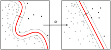
The main linear technique for dimensionality reduction, principal component analysis, performs a linear mapping of the data to a lower-dimensional space in such a way that the variance of the data in the low-dimensional representation is maximized. In practice, the covariance (and sometimes the correlation) matrix of the data is constructed and the eigenvectors on this matrix are computed. The eigenvectors that correspond to the largest eigenvalues (the principal components) can now be used to reconstruct a large fraction of the variance of the original data. Moreover, the first few eigenvectors can often be interpreted in terms of the large-scale physical behavior of the system. The original space (with dimension of the number of points) has been reduced (with data loss, but hopefully retaining the most important variance) to the space spanned by a few eigenvectors.
Kernel PCA
Principal component analysis can be employed in a nonlinear way by means of the kernel trick. The resulting technique is capable of constructing nonlinear mappings that maximize the variance in the data. The resulting technique is entitled kernel PCA.
Graph-based kernel PCA
Other prominent nonlinear techniques include manifold learning techniques such as Isomap, locally linear embedding (LLE), Hessian LLE, Laplacian eigenmaps, and local tangent space alignment (LTSA). These techniques construct a low-dimensional data representation using a cost function that retains local properties of the data, and can be viewed as defining a graph-based kernel for Kernel PCA.
More recently, techniques have been proposed that, instead of defining a fixed kernel, try to learn the kernel using semidefinite programming. The most prominent example of such a technique is maximum variance unfolding (MVU). The central idea of MVU is to exactly preserve all pairwise distances between nearest neighbors (in the inner product space), while maximizing the distances between points that are not nearest neighbors.
An alternative approach to neighborhood preservation is through the minimization of a cost function that measures differences between distances in the input and output spaces. Important examples of such techniques include: classical multidimensional scaling, which is identical to PCA; Isomap, which uses geodesic distances in the data space; diffusion maps, which use diffusion distances in the data space; t-distributed stochastic neighbor embedding (t-SNE), which minimizes the divergence between distributions over pairs of points; and curvilinear component analysis.
A different approach to nonlinear dimensionality reduction is through the use of autoencoders, a special kind of feed-forward neural networks with a bottle-neck hidden layer.[6] The training of deep encoders is typically performed using a greedy layer-wise pre-training (e.g., using a stack of restricted Boltzmann machines) that is followed by a finetuning stage based on backpropagation.
Linear discriminant analysis (LDA)
Linear discriminant analysis (LDA) is a generalization of Fisher's linear discriminant, a method used in statistics, pattern recognition and machine learning to find a linear combination of features that characterizes or separates two or more classes of objects or events.
Generalized discriminant analysis (GDA)
GDA deals with nonlinear discriminant analysis using kernel function operator. The underlying theory is close to the support vector machines (SVM) insofar as the GDA method provides a mapping of the input vectors into high-dimensional feature space.[7][8] Similar to LDA, the objective of GDA is to find a projection for the features into a lower dimensional space by maximizing the ratio of between-class scatter to within-class scatter.
Dimension reduction
For high-dimensional datasets (i.e. with number of dimensions more than 10), dimension reduction is usually performed prior to applying a K-nearest neighbors algorithm (k-NN) in order to avoid the effects of the curse of dimensionality. [9]
Feature extraction and dimension reduction can be combined in one step using principal component analysis (PCA), linear discriminant analysis (LDA), or canonical correlation analysis (CCA) techniques as a pre-processing step followed by clustering by K-NN on feature vectors in reduced-dimension space. In machine learning this process is also called low-dimensional embedding.[10]
For very-high-dimensional datasets (e.g. when performing similarity search on live video streams, DNA data or high-dimensional Time series) running a fast approximate K-NN search using locality sensitive hashing, random projection,[11] "sketches" [12] or other high-dimensional similarity search techniques from the VLDB toolbox might be the only feasible option.
Advantages of dimensionality reduction
- It reduces the time and storage space required.
- Removal of multi-collinearity improves the performance of the machine learning model.
- It becomes easier to visualize the data when reduced to very low dimensions such as 2D or 3D.
Applications
A dimensionality reduction technique that is sometimes used in neuroscience is maximally informative dimensions, which finds a lower-dimensional representation of a dataset such that as much information as possible about the original data is preserved.
See also
| Recommender systems |
|---|
| Concepts |
| Methods and challenges |
| Implementations |
| Research |
- Nearest neighbor search
- MinHash
- Information gain in decision trees
- Semidefinite embedding
- Multifactor dimensionality reduction
- Multilinear subspace learning
- Multilinear PCA
- Random projection
- Singular value decomposition
- Latent semantic analysis
- Semantic mapping
- Topological data analysis
- Locality sensitive hashing
- Sufficient dimension reduction
- Data transformation (statistics)
- Weighted correlation network analysis
- Hyperparameter optimization
Notes
- ↑ Roweis, S. T.; Saul, L. K. (2000). "Nonlinear Dimensionality Reduction by Locally Linear Embedding". Science. 290 (5500): 2323–2326. doi:10.1126/science.290.5500.2323. PMID 11125150.
- ↑ Pudil, P.; Novovičová, J. (1998). "Novel Methods for Feature Subset Selection with Respect to Problem Knowledge". In Liu, Huan; Motoda, Hiroshi. Feature Extraction, Construction and Selection. p. 101. doi:10.1007/978-1-4615-5725-8_7. ISBN 978-1-4613-7622-4.
- ↑ Samet, H. (2006) Foundations of Multidimensional and Metric Data Structures. Morgan Kaufmann. ISBN 0-12-369446-9
- ↑ C. Ding, , X. He , H. Zha , H.D. Simon, Adaptive Dimension Reduction for Clustering High Dimensional Data,Proceedings of International Conference on Data Mining, 2002
- ↑ Lu, Haiping; Plataniotis, K.N.; Venetsanopoulos, A.N. (2011). "A Survey of Multilinear Subspace Learning for Tensor Data" (PDF). Pattern Recognition. 44 (7): 1540–1551. doi:10.1016/j.patcog.2011.01.004.
- ↑ Hongbing Hu, Stephen A. Zahorian, (2010) "Dimensionality Reduction Methods for HMM Phonetic Recognition," ICASSP 2010, Dallas, TX
- ↑ G. Baudat, F. Anouar (2000). Generalized discriminant analysis using a kernel approach Neural computation, 12(10), 2385-2404.
- ↑ M. Haghighat, S. Zonouz, & M. Abdel-Mottaleb (2015). CloudID: Trustworthy Cloud-based and Cross-Enterprise Biometric Identification. Expert Systems with Applications, 42(21), 7905–7916.
- ↑ Kevin Beyer , Jonathan Goldstein , Raghu Ramakrishnan , Uri Shaft (1999) "When is “nearest neighbor” meaningful?". Database Theory—ICDT99, 217-235
- ↑ Shaw, B.; Jebara, T. (2009). "Structure preserving embedding". Proceedings of the 26th Annual International Conference on Machine Learning - ICML '09 (PDF). p. 1. doi:10.1145/1553374.1553494. ISBN 9781605585161.
- ↑ Bingham, E.; Mannila, H. (2001). "Random projection in dimensionality reduction". Proceedings of the seventh ACM SIGKDD international conference on Knowledge discovery and data mining - KDD '01. p. 245. doi:10.1145/502512.502546. ISBN 158113391X.
- ↑ Shasha, D High (2004) Performance Discovery in Time Series Berlin: Springer. ISBN 0-387-00857-8
References
- Fodor,I. (2002) "A survey of dimension reduction techniques". Center for Applied Scientific Computing, Lawrence Livermore National, Technical Report UCRL-ID-148494
- Cunningham, P. (2007) "Dimension Reduction" University College Dublin, Technical Report UCD-CSI-2007-7
- Zahorian, Stephen A.; Hu, Hongbing (2011). "Nonlinear Dimensionality Reduction Methods for Use with Automatic Speech Recognition". Speech Technologies. doi:10.5772/16863. ISBN 978-953-307-996-7.
- Lakshmi Padmaja, Dhyaram; Vishnuvardhan, B (18 August 2016). "Comparative Study of Feature Subset Selection Methods for Dimensionality Reduction on Scientific Data": 31–34. doi:10.1109/IACC.2016.16. Retrieved 7 October 2016.
External links
- JMLR Special Issue on Variable and Feature Selection
- ELastic MAPs
- Locally Linear Embedding
- A Global Geometric Framework for Nonlinear Dimensionality Reduction