Inverse function
| Function | |||||||||||||||||||||||||||||
|---|---|---|---|---|---|---|---|---|---|---|---|---|---|---|---|---|---|---|---|---|---|---|---|---|---|---|---|---|---|
| x ↦ f (x) | |||||||||||||||||||||||||||||
| By domain and codomain | |||||||||||||||||||||||||||||
|
|||||||||||||||||||||||||||||
| Classes/properties | |||||||||||||||||||||||||||||
| Constant · Identity · Linear · Polynomial · Rational · Algebraic · Analytic · Smooth · Continuous · Measurable · Injective · Surjective · Bijective | |||||||||||||||||||||||||||||
| Constructions | |||||||||||||||||||||||||||||
| Restriction · Composition · λ · Inverse | |||||||||||||||||||||||||||||
| Generalizations | |||||||||||||||||||||||||||||
| Partial · Multivalued · Implicit | |||||||||||||||||||||||||||||
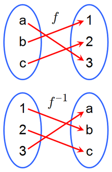
In mathematics, an inverse function is a function that "reverses" another function: if the function f applied to an input x gives a result of y, then applying its inverse function g to y gives the result x, and vice versa. i.e., f(x) = y if and only if g(y) = x.[1][2]
As a simple example, consider the real-valued function of a real variable given by f(x) = 5x − 7. Thinking of this as a step-by-step procedure (namely, take a number x, multiply it by 5, then subtract 7 from the result), to reverse this and get x back from some output value, say y, we should undo each step in reverse order. In this case that means that we should add 7 to y and then divide the result by 5. In functional notation this inverse function would be given by,

With y = 5x − 7 we have that f(x) = y and g(y) = x.
Not all functions have inverse functions. In order for a function f: X → Y to have an inverse,[3] it must have the property that for every y in Y there must be one, and only one x in X so that f(x) = y. This property ensures that a function g: Y → X will exist having the necessary relationship with f.
Definitions
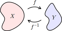
Let f be a function whose domain is the set X, and whose image (range) is the set Y. Then f is invertible if there exists a function g with domain Y and image X, with the property:

If f is invertible, the function g is unique,[4] which means that there is exactly one function g satisfying this property (no more, no less). That function g is then called the inverse of f, and is usually denoted as f −1.[5]
Stated otherwise, a function is invertible if and only if its inverse relation is a function on the range Y, in which case the inverse relation is the inverse function.[6]
Not all functions have an inverse. For a function to have an inverse, each element y ∈ Y must correspond to no more than one x ∈ X; a function f with this property is called one-to-one or an injection. If f −1 is to be a function on Y, then each element y ∈ Y must correspond to some x ∈ X. Functions with this property are called surjections. This property is satisfied by definition if Y is the image (range) of f, but may not hold in a more general context. To be invertible a function must be both an injection and a surjection. Such functions are called bijections. The inverse of an injection f: X → Y that is not a bijection, that is, a function that is not a surjection, is only a partial function on Y, which means that for some y ∈ Y, f −1(y) is undefined. If a function f is invertible, then both it and its inverse function f−1 are bijections.
There is another convention used in the definition of functions. This can be referred to as the "set-theoretic" or "graph" definition using ordered pairs in which a codomain is never referred to.[7] Under this convention all functions are surjections,[8] and so, being a bijection simply means being an injection. Authors using this convention may use the phrasing that a function is invertible if and only if it is an injection.[9] The two conventions need not cause confusion as long as it is remembered that in this alternate convention the codomain of a function is always taken to be the range of the function.
Example: squaring and square root functions
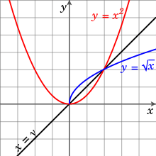
The function f:ℝ → [0,∞) given by f(x) = x2 is not injective since each possible result y (except 0) corresponds to two different starting points in X – one positive and one negative, and so this function is not invertible. With this type of function it is impossible to deduce an input from its output. Such a function is called non-injective or, in some applications, information-losing.
If the domain of the function is restricted to the nonnegative reals, that is, the function is redefined to be f: [0, ∞) → [0, ∞) with the same rule as before, then the function is bijective and so, invertible.[10] The inverse function here is called the (positive) square root function.
Inverses and composition
If f is an invertible function with domain X and range Y, then
- , for every


Using the composition of functions we can rewrite this statement as follows:

where idX is the identity function on the set X; that is, the function that leaves its argument unchanged. In category theory, this statement is used as the definition of an inverse morphism.
Considering function composition helps to understand the notation f −1. Repeatedly composing a function with itself is called iteration. If f is applied n times, starting with the value x, then this is written as f n(x); so f 2(x) = f (f (x)), etc. Since f −1(f (x)) = x, composing f −1 and f n yields f n−1, "undoing" the effect of one application of f.
Note on notation
While the notation f −1(x) might be misunderstood, (f(x))−1 certainly denotes the multiplicative inverse of f(x) and has nothing to do with the inverse function of f.
In keeping with the general notation, some authors use expressions like sin−1(x) to denote the inverse of the sine function applied to x (actually a partial inverse; see below)[11] Other authors feel that this may be confused with the notation for the multiplicative inverse of sin (x), which can be denoted as (sin (x))−1. To avoid any confusion, an inverse trigonometric function is often indicated by the prefix "arc" (for Latin arcus).[12][13] For instance, the inverse of the sine function is typically called the arcsine function, written as arcsin(x).[12][13] Similarly, the inverse of a hyperbolic function is indicated by the prefix "ar" (for Latin area).[13] For instance, the inverse of the hyperbolic sine function is typically written as arsinh(x).[13] Other inverse special functions are sometimes prefixed with the prefix "inv" if the ambiguity of the f −1 notation should be avoided.[13]
Properties
Since a function is a special type of binary relation, many of the properties of an inverse function correspond to properties of inverse relations.
Uniqueness
If an inverse function exists for a given function f, then it is unique.[14] This follows since the inverse function must be the inverse relation which is completely determined by f.
Symmetry
There is a symmetry between a function and its inverse. Specifically, if f is an invertible function with domain X and range Y, then its inverse f −1 has domain Y and range X, and the inverse of f −1 is the original function f. In symbols, for functions f:X → Y and f−1:Y → X,[14]
- and


This statement is an consequence of the implication that for f to be invertible it must be bijective. The involutory nature of the inverse can be concisely expressed by[15]

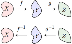
The inverse of a composition of functions is given by[16]

Notice that the order of g and f have been reversed; to undo f followed by g, we must first undo g and then undo f.
For example, let f(x) = 3x and let g(x) = x + 5. Then the composition g ∘ f is the function that first multiplies by three and then adds five,

To reverse this process, we must first subtract five, and then divide by three,

This is the composition (f −1 ∘ g −1)(x).
Self-inverses
If X is a set, then the identity function on X is its own inverse:

More generally, a function f : X → X is equal to its own inverse if and only if the composition f ∘ f is equal to idX. Such a function is called an involution.
Inverses in calculus
Single-variable calculus is primarily concerned with functions that map real numbers to real numbers. Such functions are often defined through formulas, such as:

A surjective function f from the real numbers to the real numbers possesses an inverse as long as it is one-to-one, i.e. as long as the graph of y = f(x) has, for each possible y value only one corresponding x value, and thus passes the horizontal line test.
The following table shows several standard functions and their inverses:
Function f(x) Inverse f −1(y) Notes x + a y − a a − x a − y mx y/m m ≠ 0 1/x (i.e. x−1) 1/y (i.e. y−1) x, y ≠ 0 x2 √y (i.e. y1/2) x, y ≥ 0 only x3 3√y (i.e. y1/3) no restriction on x and y xp p√y (i.e. y1/p) x, y ≥ 0 in general, p ≠ 0 2x lb y y > 0 ex ln y y > 0 10x log y y > 0 ax loga y y > 0 and a > 0 trigonometric functions inverse trigonometric functions various restrictions (see table below) hyperbolic functions inverse hyperbolic functions various restrictions
Formula for the inverse
One approach to finding a formula for f −1, if it exists, is to solve the equation y = f(x) for x.[17] For example, if f is the function

then we must solve the equation y = (2x + 8)3 for x:
![{\begin{aligned}y&=(2x+8)^{3}\\{\sqrt[{3}]{y}}&=2x+8\\{\sqrt[{3}]{y}}-8&=2x\\{\dfrac {{\sqrt[{3}]{y}}-8}{2}}&=x.\end{aligned}}](../I/m/3107b63d271dd3e5b2f928a036c04525c896fbda.svg)
Thus the inverse function f −1 is given by the formula
![f^{-1}(y)={\dfrac {{\sqrt[{3}]{y}}-8}{2}}.](../I/m/a149deb3a34cae86402ef07eaa54bd52b5e3b9ae.svg)
Sometimes the inverse of a function cannot be expressed by a formula with a finite number of terms. For example, if f is the function

then f is a bijection, and therefore possesses an inverse function f −1. The formula for this inverse has an infinite number of terms:
![{\displaystyle f^{-1}(y)=\displaystyle \sum _{n=1}^{\infty }{\frac {y^{\frac {n}{3}}}{n!}}\lim _{\theta \to 0}\left({\frac {\mathrm {d} ^{\,n-1}}{\mathrm {d} \theta ^{\,n-1}}}\left({\frac {\theta }{\sqrt[{3}]{\theta -\sin(\theta )}}}\right)^{n}\right).}](../I/m/86552a8adf715c569b60d0065e442933d28d5169.svg)
Graph of the inverse
If f is invertible, then the graph of the function

is the same as the graph of the equation

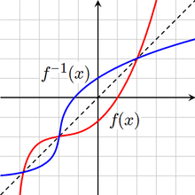
This is identical to the equation y = f(x) that defines the graph of f, except that the roles of x and y have been reversed. Thus the graph of f −1 can be obtained from the graph of f by switching the positions of the x and y axes. This is equivalent to reflecting the graph across the line y = x.[18]
Inverses and derivatives
A continuous function f is invertible on its range (image) if and only if it is either strictly increasing or decreasing (with no local maxima or minima). For example, the function

is invertible, since the derivative f′(x) = 3x2 + 1 is always positive.
If the function f is differentiable on an interval I and f′(x) ≠ 0 for each x ∈ I, then the inverse f −1 will be differentiable on f(I).[19] If y = f(x), the derivative of the inverse is given by the inverse function theorem,

Using Leibniz's notation the formula above can be written as

This result follows from the chain rule (see the article on inverse functions and differentiation).
The inverse function theorem can be generalized to functions of several variables. Specifically, a differentiable multivariable function f : Rn → Rn is invertible in a neighborhood of a point p as long as the Jacobian matrix of f at p is invertible. In this case, the Jacobian of f −1 at f(p) is the matrix inverse of the Jacobian of f at p.
Real-world examples
- Let f be the function that converts a temperature in degrees Celsius to a temperature in degrees Fahrenheit,
- then its inverse function converts degrees Fahrenheit to degrees Celsius,
- since
- for every C, and
- for all F.


- Suppose f assigns each child in a family its birth year. An inverse function would output which child was born in a given year. However, if the family children born in the same year (for instance, twins or triplets, etc.) then the output cannot be known when the input is the common birth year. As well, if a year is given in which no child was born then a child cannot be named. But if each child was born in a separate year, and if we restrict attention to the three years in which a child was born, then we do have an inverse function. For example,

- Let R be the function that leads to an x percentage rise of some quantity, and F be the function producing an x percentage fall. Applied to $100 with x = 10%, we find that applying the first function followed by the second does not restore the original value of $100, demonstrating the fact that, despite appearances, these two functions are not inverses of each other.
Generalizations
Partial inverses
Even if a function f is not one-to-one, it may be possible to define a partial inverse of f by restricting the domain. For example, the function

is not one-to-one, since x2 = (−x)2. However, the function becomes one-to-one if we restrict to the domain x ≥ 0, in which case

(If we instead restrict to the domain x ≤ 0, then the inverse is the negative of the square root of y.) Alternatively, there is no need to restrict the domain if we are content with the inverse being a multivalued function:

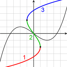
Sometimes this multivalued inverse is called the full inverse of f, and the portions (such as √x and −√x) are called branches. The most important branch of a multivalued function (e.g. the positive square root) is called the principal branch, and its value at y is called the principal value of f −1(y).
For a continuous function on the real line, one branch is required between each pair of local extrema. For example, the inverse of a cubic function with a local maximum and a local minimum has three branches (see the adjacent picture).
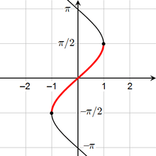
These considerations are particularly important for defining the inverses of trigonometric functions. For example, the sine function is not one-to-one, since

for every real x (and more generally sin(x + 2πn) = sin(x) for every integer n). However, the sine is one-to-one on the interval [−π/2, π/2], and the corresponding partial inverse is called the arcsine. This is considered the principal branch of the inverse sine, so the principal value of the inverse sine is always between −π/2 and π/2. The following table describes the principal branch of each inverse trigonometric function:[20]
function Range of usual principal value arcsin −π/2 ≤ sin−1(x) ≤ π/2 arccos 0 ≤ cos−1(x) ≤ π arctan −π/2 < tan−1(x) < π/2 arccot 0 < cot−1(x) < π arcsec 0 ≤ sec−1(x) ≤ π arccsc −π/2 ≤ csc−1(x) ≤ π/2
Left and right inverses
If f: X → Y, a left inverse for f (or retraction of f ) is a function g: Y → X such that

That is, the function g satisfies the rule
- If , then


Thus, g must equal the inverse of f on the image of f, but may take any values for elements of Y not in the image. A function f with a left inverse is necessarily injective. In classical mathematics, every injective function f with a nonempty domain necessarily has a left inverse; however, this may fail in constructive mathematics. For instance, a left inverse of the inclusion {0,1} → R of the two-element set in the reals violates indecomposability by giving a retraction of the real line to the set {0,1} .
A right inverse for f (or section of f ) is a function h: Y → X such that

That is, the function h satisfies the rule
- If , then


Thus, h(y) may be any of the elements of X that map to y under f. A function f has a right inverse if and only if it is surjective (though constructing such an inverse in general requires the axiom of choice).
An inverse which is both a left and right inverse must be unique. However, if g is a left inverse for f, then g may or may not be a right inverse for f; and if g is a right inverse for f, then g is not necessarily a left inverse for f. For example, let f: R → [0, ∞) denote the squaring map, such that f(x) = x2 for all x in R, and let g: [0, ∞) → R denote the square root map, such that g(x) = √x for all x ≥ 0. Then f(g(x)) = x for all x in [0, ∞); that is, g is a right inverse to f. However, g is not a left inverse to f, since, e.g., g(f(−1)) = 1 ≠ −1.
Preimages
If f: X → Y is any function (not necessarily invertible), the preimage (or inverse image) of an element y ∈ Y is the set of all elements of X that map to y:

The preimage of y can be thought of as the image of y under the (multivalued) full inverse of the function f.
Similarly, if S is any subset of Y, the preimage of S is the set of all elements of X that map to S:

For example, take a function f: R → R, where f: x ↦ x2. This function is not invertible for reasons discussed above. Yet preimages may be defined for subsets of the codomain:

The preimage of a single element y ∈ Y – a singleton set {y} – is sometimes called the fiber of y. When Y is the set of real numbers, it is common to refer to f −1({y}) as a level set.
See also
- Lagrange inversion theorem, gives the Taylor series expansion of the inverse function of an analytic function
Notes
- ↑ Keisler, H. Jerome. "Differentiation" (PDF). Retrieved 2015-01-24.
§ 2.4
- ↑ Scheinerman, Edward R. (2013). Mathematics: A Discrete Introduction. Brooks/Cole. p. 173. ISBN 978-0840049421.
- ↑ It is a common practice, when no ambiguity can arise, to leave off the term function and just refer to an inverse.
- ↑ Devlin 2004, p. 101, Theorem 4.5.1
- ↑ Not to be confused with numerical exponentiation such as taking the multiplicative inverse of a nonzero real number.
- ↑ Smith, Eggen & St. Andre 2006, p. 202, Theorem 4.9
- ↑ Wolf 1998, p.198
- ↑ So this term is never used in this convention
- ↑ Fletcher & Patty 1988, p. 116 Theorem 5.1
- ↑ Lay 2006, p.69 Example 7.24
- ↑ .Thomas 1972, pp. 304-309
- 1 2 Korn, Grandino Arthur; Korn, Theresa M. (2000) [1961]. "21.2.-4. Inverse Trigonometric Functions". Mathematical handbook for scientists and engineers: Definitions, theorems, and formulars for reference and review (3 ed.). Mineola, New York, USA: Dover Publications, Inc. p. 811;. ISBN 978-0-486-41147-7.
- 1 2 3 4 5 Oldham, Keith B.; Myland, Jan C.; Spanier, Jerome (2009) [1987]. An Atlas of Functions: with Equator, the Atlas Function Calculator (2 ed.). Springer Science+Business Media, LLC. doi:10.1007/978-0-387-48807-3. ISBN 978-0-387-48806-6. LCCN 2008937525.
- 1 2 Wolf 1998, p. 208 Theorem 7.2
- ↑ Smith, Eggen & St. Andre 2006, pg. 141 Theorem 3.3(a)
- ↑ Lay 2006, p. 71 Theorem 7.26
- ↑ Devlin 2004, p. 101
- ↑ Briggs & Cochran 2011, pp. 28-29
- ↑ Lay 2006, p. 246 Theorem 26.10
- ↑ Briggs & Cochran 2011, pp. 39-42
References
- Briggs, William; Cochran, Lyle (2011), Calculus / Early Transcendentals Single Variable, Addison-Wesley, ISBN 978-0-321-66414-3
- Devlin, Keith (2004), Sets, Functions, and Logic / An Introduction to Abstract Mathematics (3rd ed.), Chapman & Hall / CRC Mathematics, ISBN 978-1-58488-449-1
- Fletcher, Peter; Patty, C. Wayne (1988), Foundations of Higher Mathematics, PWS-Kent, ISBN 0-87150-164-3
- Lay, Steven R. (2006), Analysis / With an Introduction to Proof (4th ed.), Pearson / Prentice Hall, ISBN 978-0-13-148101-5
- Smith, Douglas; Eggen, Maurice; St. Andre, Richard (2006). A Transition to Advanced Mathematics (6 ed.). Thompson Brooks/Cole. ISBN 978-0-534-39900-9.
- Thomas, Jr., George B. (1972). Calculus and Analytic Geometry Part 1: Functions of One Variable and Analytic Geometry (Alternate ed.). Addison-Wesley.
- Wolf, Robert S. (1998), Proof, Logic, and Conjecture / The Mathematician's Toolbox, W. H. Freeman and Co., ISBN 978-0-7167-3050-7
Further reading
- Spivak, Michael (1994). Calculus (3 ed.). Publish or Perish. ISBN 0-914098-89-6.
- Stewart, James (2002). Calculus (5 ed.). Brooks Cole. ISBN 978-0-534-39339-7.
External links
- Hazewinkel, Michiel, ed. (2001), "Inverse function", Encyclopedia of Mathematics, Springer, ISBN 978-1-55608-010-4
- Wikibook: Functions
- Wolfram Mathworld: Inverse Function