Klee–Minty cube

The Klee–Minty cube or Klee–Minty polytope (named after Victor Klee and George J. Minty) is a unit hypercube of variable dimension whose corners have been perturbed. Klee and Minty demonstrated that George Dantzig's simplex algorithm has poor worst-case performance when initialized at one corner of their "squashed cube".
In particular, many optimization algorithms for linear optimization exhibit poor performance when applied to the Klee–Minty cube. In 1973 Klee and Minty showed that Dantzig's simplex algorithm was not a polynomial-time algorithm when applied to their cube.[1] Later, modifications of the Klee–Minty cube have shown poor behavior both for other basis-exchange pivoting algorithms and also for interior-point algorithms.
Description of the cube
The Klee–Minty cube was originally specified with a parameterized system of linear inequalities, with the dimension as the parameter. When the dimension is two, the "cube" is a squashed square. When the dimension is three, the "cube" is a squashed cube. Illustrations of the "cube" have appeared besides algebraic descriptions.[2][3]
The Klee–Minty polytope is given by[4]

This has D variables, D constraints other than the D non-negativity constraints, and 2D vertices, just as a D-dimensional hypercube does. If the objective function to be maximized is

and if the initial vertex for the simplex algorithm is the origin, then the algorithm as formulated by Dantzig visits all 2D vertices, finally reaching the optimal vertex

Computational complexity
The Klee–Minty cube has been used to analyze the performance of many algorithms, both in the worst case and on average. The time complexity of an algorithm counts the number of arithmetic operations sufficient for the algorithm to solve the problem. For example, Gaussian elimination requires on the order of D3 operations, and so it is said to have polynomial time-complexity, because its complexity is bounded by a cubic polynomial. There are examples of algorithms that do not have polynomial-time complexity. For example, a generalization of Gaussian elimination called Buchberger's algorithm has for its complexity an exponential function of the problem data (the degree of the polynomials and the number of variables of the multivariate polynomials). Because exponential functions eventually grow much faster than polynomial functions, an exponential complexity implies that an algorithm has slow performance on large problems.
Worst case
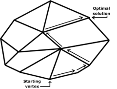
In mathematical optimization, the Klee–Minty cube is an example that shows the worst-case computational complexity of many algorithms of linear optimization. It is a deformed cube with exactly 2D corners in dimension D. Klee and Minty showed that Dantzig's simplex algorithm visits all corners of a (perturbed) cube in dimension D in the worst case.[1][5][6]
Modifications of the Klee–Minty construction showed similar exponential time complexity for other pivoting rules of simplex type, which maintain primal feasibility, such as Bland's rule.[7][8][9] Another modification showed that the criss-cross algorithm, which does not maintain primal feasibility, also visits all the corners of a modified Klee–Minty cube.[6][10][11] Like the simplex algorithm, the criss-cross algorithm visits all 8 corners of the three-dimensional cube in the worst case.
Path-following algorithms
Further modifications of the Klee–Minty cube have shown poor performance of central-path–following algorithms for linear optimization, in that the central path comes arbitrarily close to each of the corners of a cube. This "vertex-stalking" performance is surprising, because such path-following algorithms have polynomial-time complexity for linear optimization.[2][12]
Average case
The Klee–Minty cube has also inspired research on average-case complexity. When eligible pivots are made randomly (and not by the rule of steepest descent), Dantzig's simplex algorithm needs on average quadratically many steps (on the order of O(D2).[3] Standard variants of the simplex algorithm takes on average D steps for a cube.[13] When it is initialized at a random corner of the cube, the criss-cross algorithm visits only D additional corners, however, according to a 1994 paper by Fukuda and Namiki.[14][15] Both the simplex algorithm and the criss-cross algorithm visit exactly 3 additional corners of the three-dimensional cube on average.
See also
Notes
- 1 2 Klee & Minty (1972)
- 1 2 Deza, Nematollahi & Terlaky (2008)
- 1 2 Gartner & Ziegler (1994)
- ↑ Greenberg, Harvey J., Klee-Minty Polytope Shows Exponential Time Complexity of Simplex Method University of Colorado at Denver (1997) PDF download
- ↑ Murty (1983, 14.2 Worst-case computational complexity, pp. 434–437)
- 1 2 Terlaky & Zhang (1993)
- ↑ Bland, Robert G. (May 1977). "New finite pivoting rules for the simplex method". Mathematics of Operations Research. 2 (2): 103–107. doi:10.1287/moor.2.2.103. JSTOR 3689647. MR 459599.
- ↑ Murty (1983, Chapter 10.5, pp. 331–333; problem 14.8, p. 439) describes Bland's rule.
- ↑ Murty (1983, Problem 14.3, p. 438; problem 14.8, p. 439) describes the worst-case complexity of Bland's rule.
- ↑ Roos (1990)
- ↑ Fukuda & Terlaky (1997)
- ↑ Megiddo & Shub (1989)
- ↑ More generally, for the simplex algorithm, the expected number of steps is proportional to D for linear-programming problems that are randomly drawn from the Euclidean unit sphere, as proved by Borgwardt and by Smale.
Borgwardt (1987): Borgwardt, Karl-Heinz (1987). The simplex method: A probabilistic analysis. Algorithms and Combinatorics (Study and Research Texts). 1. Berlin: Springer-Verlag. pp. xii+268. ISBN 3-540-17096-0. MR 868467.
- ↑ Fukuda & Namiki (1994, p. 367)
- ↑ Fukuda & Terlaky (1997, p. 385)
References
- Deza, Antoine; Nematollahi, Eissa; Terlaky, Tamás (May 2008). "How good are interior point methods? Klee–Minty cubes tighten iteration-complexity bounds". Mathematical Programming. 113 (1): 1–14. doi:10.1007/s10107-006-0044-x. MR 2367063.
- Fukuda, Komei; Namiki, Makoto (March 1994). "On extremal behaviors of Murty's least index method". Mathematical Programming. 64 (1): 365–370. doi:10.1007/BF01582581. MR 1286455.
- Fukuda, Komei; Terlaky, Tamás (1997). Thomas M. Liebling and Dominique de Werra, eds. "Criss-cross methods: A fresh view on pivot algorithms". Mathematical Programming: Series B. Amsterdam: North-Holland Publishing Co., number 1—3. 79 (Papers from the 16th International Symposium on Mathematical Programming held in Lausanne, 1997): 369–395. doi:10.1007/BF02614325. MR 1464775. Postscript preprint.
- Gartner, B.; Ziegler, G. M. (1994). "Randomized simplex algorithms on Klee-Minty cubes". Foundations of Computer Science, Annual IEEE Symposium on. IEEE (35th Annual Symposium on Foundations of Computer Science (FOCS 1994)): 502–510. doi:10.1109/SFCS.1994.365741.
- Klee, Victor; Minty, George J. (1972). "How good is the simplex algorithm?". In Shisha, Oved. Inequalities III (Proceedings of the Third Symposium on Inequalities held at the University of California, Los Angeles, Calif., September 1–9, 1969, dedicated to the memory of Theodore S. Motzkin). New York-London: Academic Press. pp. 159–175. MR 332165.
- Megiddo, Nimrod; Shub, Michael (February 1989). "Boundary Behavior of Interior Point Algorithms in Linear Programming". Mathematics of Operations Research. 14 (1): 97–146. doi:10.1287/moor.14.1.97. JSTOR 3689840. MR 984561.
- Murty, Katta G. (1983). Linear programming. New York: John Wiley & Sons. pp. xix+482. ISBN 0-471-09725-X. MR 720547.
- Roos, C. (1990). "An exponential example for Terlaky's pivoting rule for the criss-cross simplex method". Mathematical Programming. Series A. 46 (1): 79–84. doi:10.1007/BF01585729. MR 1045573.
- Terlaky, Tamás; Zhang, Shu Zhong (1993). "Pivot rules for linear programming: A Survey on recent theoretical developments". Annals of Operations Research. Springer Netherlands. 46–47 (Degeneracy in optimization problems; number 1): 203–233. CiteSeerX 10.1.1.36.7658
 . doi:10.1007/BF02096264. ISSN 0254-5330. MR 1260019.
External links
Algebraic description with illustration
The first two links have both an algebraic construction and a picture of a three-dimensional Klee–Minty cube:
- Deza, Antoine; Nematollahi, Eissa; Terlaky, Tamás (May 2008). "How good are interior point methods? Klee–Minty cubes tighten iteration-complexity bounds". Mathematical Programming. 113 (1): 1–14. doi:10.1007/s10107-006-0044-x. MR 2367063. (subscription required). pdf version at Professor Deza's homepage.
- Gartner, B.; Ziegler, G. M. (1994). "Randomized simplex algorithms on Klee-Minty cubes". Foundations of Computer Science, Annual IEEE Symposium on. IEEE (35th Annual Symposium on Foundations of Computer Science (FOCS 1994)): 502–510. doi:10.1109/SFCS.1994.365741. IEEE mis-spells the name "Gärnter" as "Gartner" (sic.).
Pictures with no linear system
- Articles of E. Nematollahi, which discuss the Klee-Minty cube with illustrations.
- A picture of a Klee-Minty cube showing a simplex-algorithm path (automatic translation of German) by Günter Ziegler. The picture in the second half of the page.
|  | |||||||||||||||||||||||||||
|
| ||||||||||||||||||||||||||||
| ||||||||||||||||||||||||||||
| ||||||||||||||||||||||||||||