Log-logistic distribution
|
Probability density function 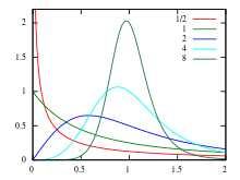 values of as shown in legend | |
|
Cumulative distribution function 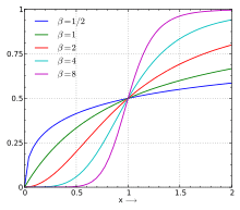 values of as shown in legend | |
| Parameters |
scale shape |
|---|---|
| Support | |
| CDF | |
| Mean |
if , else undefined |
| Median | |
| Mode |
if , 0 otherwise |
| Variance | See main text |


In probability and statistics, the log-logistic distribution (known as the Fisk distribution in economics) is a continuous probability distribution for a non-negative random variable. It is used in survival analysis as a parametric model for events whose rate increases initially and decreases later, for example mortality rate from cancer following diagnosis or treatment. It has also been used in hydrology to model stream flow and precipitation, and in economics as a simple model of the distribution of wealth or income.
The log-logistic distribution is the probability distribution of a random variable whose logarithm has a logistic distribution. It is similar in shape to the log-normal distribution but has heavier tails. Unlike the log-normal, its cumulative distribution function can be written in closed form.
Characterisation
There are several different parameterizations of the distribution in use. The one shown here gives reasonably interpretable parameters and a simple form for the cumulative distribution function.[1][2] The parameter is a scale parameter and is also the median of the distribution. The parameter is a shape parameter. The distribution is unimodal when and its dispersion decreases as increases.
The cumulative distribution function is

where , ,


The probability density function is

Alternative parameterization
An alternative parametrization is given by the pair in analogy with the logistic distribution:


Properties
Moments
The th raw moment exists only when when it is given by[3][4]


where B() is the beta function. Expressions for the mean, variance, skewness and kurtosis can be derived from this. Writing for convenience, the mean is


and the variance is

Explicit expressions for the skewness and kurtosis are lengthy.[5] As tends to infinity the mean tends to , the variance and skewness tend to zero and the excess kurtosis tends to 6/5 (see also related distributions below).

Quantiles
The quantile function (inverse cumulative distribution function) is :

It follows that the median is , the lower quartile is and the upper quartile is .


Applications
Survival analysis
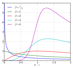
The log-logistic distribution provides one parametric model for survival analysis. Unlike the more commonly used Weibull distribution, it can have a non-monotonic hazard function: when the hazard function is unimodal (when ≤ 1, the hazard decreases monotonically). The fact that the cumulative distribution function can be written in closed form is particularly useful for analysis of survival data with censoring.[6] The log-logistic distribution can be used as the basis of an accelerated failure time model by allowing to differ between groups, or more generally by introducing covariates that affect but not by modelling as a linear function of the covariates.[7]


The survival function is
![S(t)=1-F(t)=[1+(t/\alpha )^{{\beta }}]^{{-1}},\,](../I/m/fbf9d6e8b7c075f857d131d44f7ac07c67e43eb7.svg)
and so the hazard function is

Hydrology

The log-logistic distribution has been used in hydrology for modelling stream flow rates and precipitation.[1][2]
Extreme values like maximum one-day rainfall and river discharge per month or per year often follow a log-normal distribution.[8] The log-normal distribution, however, needs a numeric approximation. As the log-logistic distribution, which can be solved analytically, is similar to the log-normal distribution, it can be used instead.
The blue picture illustrates an example of fitting the log-logistic distribution to ranked maximum one-day October rainfalls and it shows the 90% confidence belt based on the binomial distribution. The rainfall data are represented by the plotting position r/(n+1) as part of the cumulative frequency analysis.
Economics
The log-logistic has been used as a simple model of the distribution of wealth or income in economics, where it is known as the Fisk distribution.[9] Its Gini coefficient is .[10]

Networking
The log-logistic has been used as a model for the period of time beginning when some data leaves a software user application in a computer and the response is received by the same application after travelling through and being processed by other computers, applications, and network segments, most or all of them without hard real-time guarantees (for example, when an application is displaying data coming from a remote sensor connected to the Internet). It has been shown to be a more accurate probabilistic model for that than the log-normal distribution or others, as long as abrupt changes of regime in the sequences of those times are properly detected.[11]
Related distributions
- If then
- (Dagum distribution)
- (Singh-Maddala distribution)
- Beta prime distribution
- If X has a log-logistic distribution with scale parameter and shape parameter then Y = log(X) has a logistic distribution with location parameter and scale parameter .
- As the shape parameter of the log-logistic distribution increases, its shape increasingly resembles that of a (very narrow) logistic distribution. Informally, as →∞,


- The log-logistic distribution with shape parameter and scale parameter is the same as the generalized Pareto distribution with location parameter , shape parameter and scale parameter


- The addition of another parameter (a shift parameter) formally results in a shifted log-logistic distribution, but this is usually considered in a different parameterization so that the distribution can be bounded above or bounded below.
Generalizations
Several different distributions are sometimes referred to as the generalized log-logistic distribution, as they contain the log-logistic as a special case.[10] These include the Burr Type XII distribution (also known as the Singh-Maddala distribution) and the Dagum distribution, both of which include a second shape parameter. Both are in turn special cases of the even more general generalized beta distribution of the second kind. Another more straightforward generalization of the log-logistic is the shifted log-logistic distribution.
See also
References
- 1 2 Shoukri, M.M.; Mian, I.U.M.; Tracy, D.S. (1988), "Sampling Properties of Estimators of the Log-Logistic Distribution with Application to Canadian Precipitation Data", The Canadian Journal of Statistics, 16 (3): 223–236, doi:10.2307/3314729, JSTOR 3314729
- 1 2 Ashkar, Fahim; Mahdi, Smail (2006), "Fitting the log-logistic distribution by generalized moments", Journal of Hydrology, 328 (3–4): 694–703, doi:10.1016/j.jhydrol.2006.01.014
- ↑ Tadikamalla, Pandu R.; Johnson, Norman L. (1982), "Systems of Frequency Curves Generated by Transformations of Logistic Variables", Biometrika, 69 (2): 461–465, doi:10.1093/biomet/69.2.461, JSTOR 2335422
- ↑ Tadikamalla, Pandu R. (1980), "A Look at the Burr and Related Distributions", International Statistical Review, 48 (3): 337–344, doi:10.2307/1402945, JSTOR 1402945
- ↑ McLaughlin, Michael P. (2001), A Compendium of Common Probability Distributions (PDF), p. A–37, retrieved 2008-02-15
- ↑ Bennett, Steve (1983), "Log-Logistic Regression Models for Survival Data", Journal of the Royal Statistical Society, Series C, 32 (2): 165–171, doi:10.2307/2347295, JSTOR 2347295
- ↑ Collett, Dave (2003), Modelling Survival Data in Medical Research (2nd ed.), CRC press, ISBN 1-58488-325-1
- ↑ Ritzema (ed.), H.P. (1994), Frequency and Regression Analysis (PDF), Chapter 6 in: Drainage Principles and Applications, Publication 16, International Institute for Land Reclamation and Improvement (ILRI), Wageningen, The Netherlands, pp. 175–224, ISBN 90-70754-33-9
- ↑ Fisk, P.R. (1961), "The Graduation of Income Distributions", Econometrica, 29 (2): 171–185, doi:10.2307/1909287, JSTOR 1909287
- 1 2 Kleiber, C.; Kotz, S (2003), Statistical Size Distributions in Economics and Actuarial Sciences, Wiley, ISBN 0-471-15064-9
- ↑ Gago-Benítez, A.; Fernández-Madrigal J.-A., Cruz-Martín, A. (2013), Log-Logistic Modeling of Sensory Flow Delays in Networked Telerobots, IEEE Sensors 13(8), pp. 2944–2953