Inverse Gaussian distribution

Inverse Gaussian

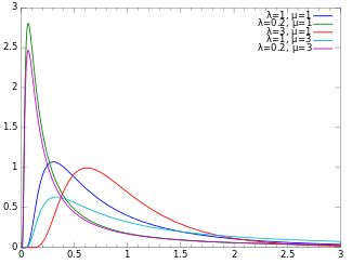
Probability density function
Parameters	$\lambda >0$ $\mu >0$
Support	$x\in (0,\infty )$
PDF	${\displaystyle \left[{\frac {\lambda }{2\pi x^{3}}}\right]^{1/2}\exp \left\{{\frac {-\lambda (x-\mu )^{2}}{2\mu ^{2}x}}\right\}}$
CDF	$\Phi \left({\sqrt {\frac {\lambda }{x}}}\left({\frac {x}{\mu }}-1\right)\right)$ $+\exp \left({\frac {2\lambda }{\mu }}\right)\Phi \left(-{\sqrt {\frac {\lambda }{x}}}\left({\frac {x}{\mu }}+1\right)\right)$ where $\Phi \left(\right)$ is the standard normal (standard Gaussian) distribution c.d.f.
Mean	$\scriptstyle \mathbf {E} [X]=\mu$ $\scriptstyle \mathbf {E} [{\frac {1}{X}}]={\frac {1}{\mu }}+{\frac {1}{\lambda }}$
Mode	$\mu \left[\left(1+{\frac {9\mu ^{2}}{4\lambda ^{2}}}\right)^{\frac {1}{2}}-{\frac {3\mu }{2\lambda }}\right]$
Variance	$\scriptstyle \mathbf {Var} [X]={\frac {\mu ^{3}}{\lambda }}$ $\scriptstyle \mathbf {Var} [{\frac {1}{X}}]={\frac {1}{\mu \lambda }}+{\frac {2}{\lambda ^{2}}}$
Skewness	$3\left({\frac {\mu }{\lambda }}\right)^{1/2}$
Ex. kurtosis	${\frac {15\mu }{\lambda }}$
MGF	${\displaystyle \exp \left[{{\frac {\lambda }{\mu }}\left(1-{\sqrt {1-{\frac {2\mu ^{2}t}{\lambda }}}}\right)}\right]}$
CF	${\displaystyle \exp \left[{{\frac {\lambda }{\mu }}\left(1-{\sqrt {1-{\frac {2\mu ^{2}\mathrm {i} t}{\lambda }}}}\right)}\right]}$

In probability theory, the inverse Gaussian distribution (also known as the Wald distribution) is a two-parameter family of continuous probability distributions with support on (0,∞).

Its probability density function is given by

${\displaystyle f(x;\mu ,\lambda )=\left[{\frac {\lambda }{2\pi x^{3}}}\right]^{1/2}\exp \left\{{\frac {-\lambda (x-\mu )^{2}}{2\mu ^{2}x}}\right\}}$

for x > 0, where $\mu >0$ is the mean and $\lambda >0$ is the shape parameter.^[1]

As λ tends to infinity, the inverse Gaussian distribution becomes more like a normal (Gaussian) distribution. The inverse Gaussian distribution has several properties analogous to a Gaussian distribution. The name can be misleading: it is an "inverse" only in that, while the Gaussian describes a Brownian Motion's level at a fixed time, the inverse Gaussian describes the distribution of the time a Brownian Motion with positive drift takes to reach a fixed positive level.

Its cumulant generating function (logarithm of the characteristic function) is the inverse of the cumulant generating function of a Gaussian random variable.

To indicate that a random variable X is inverse Gaussian-distributed with mean μ and shape parameter λ we write

$X\sim IG(\mu ,\lambda ).\,\!$

Properties

Single parameter form

The probability density function (pdf) of inverse Gaussian distribution has a single parameter form given by

${\displaystyle f(x;\mu ,\mu ^{2})={\frac {\mu }{{\sqrt {2\pi }}x^{3/2}}}\exp \left\{-{\frac {1}{2}}{\frac {(x-\mu )^{2}}{x}}\right\}.}$

In this form, the mean and variance of the distribution are equal, ${\displaystyle \mu =\sigma ^{2}.}$

Also, the cumulative distribution function (cdf) of the single parameter inverse Gaussian distribution is related to the standard normal distribution by

${\displaystyle {\begin{aligned}\mathrm {Pr} (X<x)&=\Phi (z_{1})+e^{\mu }\Phi (z_{2}),&\mathrm {for} &\quad 0<x\leq \mu ,\\\mathrm {Pr} (X>x)&=\Phi (-z_{1})-e^{\mu }\Phi (z_{2}),&\mathrm {for} &\quad x\geq \mu .\end{aligned}}}$

where ${\displaystyle z_{1}={\frac {\mu }{x^{1/2}}}-x^{1/2}}$ and ${\displaystyle z_{2}={\frac {\mu }{x^{1/2}}}+x^{1/2},}$ where the $\Phi$ is the cdf of standard normal distribution. The variables $z_{1}$ and $z_{2}$ are related to each other by the identity ${\displaystyle z_{2}^{2}=z_{1}^{2}+4\mu .}$

In the single parameter form, the MGF simplifies to

${\displaystyle M(t)=\exp[\mu (1-{\sqrt {1-2t}})].}$

An inverse Gaussian distribution in double parameter form ${\displaystyle f(x;\mu ,\lambda )}$ can be transformed into a single parameter form ${\displaystyle f(y;\mu _{0},\mu _{0}^{2})}$ by appropriate scaling ${\displaystyle y={\frac {\mu ^{2}x}{\lambda }},}$ where ${\displaystyle \mu _{0}=\mu ^{3}/\lambda .}$

The standard form of inverse Gaussian distribution is

${\displaystyle f(x;1,1)={\frac {1}{{\sqrt {2\pi }}x^{3/2}}}\exp \left\{-{\frac {1}{2}}{\frac {(x-1)^{2}}{x}}\right\}.}$

Summation

If X_i has an IG(μ₀w_i, λ₀w_i²) distribution for i = 1, 2, ..., n and all X_i are independent, then

$S=\sum _{i=1}^{n}X_{i}\sim IG\left(\mu _{0}\sum w_{i},\lambda _{0}\left(\sum w_{i}\right)^{2}\right).$

Note that

${\frac {{\textrm {Var}}(X_{i})}{{\textrm {E}}(X_{i})}}={\frac {\mu _{0}^{2}w_{i}^{2}}{\lambda _{0}w_{i}^{2}}}={\frac {\mu _{0}^{2}}{\lambda _{0}}}$

is constant for all i. This is a necessary condition for the summation. Otherwise S would not be inverse Gaussian.

Scaling

For any t > 0 it holds that

$X\sim IG(\mu ,\lambda )\,\,\,\,\,\,\Rightarrow \,\,\,\,\,\,tX\sim IG(t\mu ,t\lambda ).$

Exponential family

The inverse Gaussian distribution is a two-parameter exponential family with natural parameters -λ/(2μ²) and -λ/2, and natural statistics X and 1/X.

Differential equation

$\left\{2\mu ^{2}x^{2}f'(x)+f(x)\left(-\lambda \mu ^{2}+\lambda x^{2}+3\mu ^{2}x\right)=0,f(1)={\frac {{\sqrt {\lambda }}e^{-{\frac {\lambda (1-\mu )^{2}}{2\mu ^{2}}}}}{\sqrt {2\pi }}}\right\}$

Relationship with Brownian motion

The stochastic process X_t given by

$X_{0}=0\quad$

$X_{t}=\nu t+\sigma W_{t}\quad \quad \quad \quad$

(where W_t is a standard Brownian motion and $\nu >0$) is a Brownian motion with drift ν.

Then, the first passage time for a fixed level $\alpha >0$ by X_t is distributed according to an inverse-gaussian:

${\displaystyle T_{\alpha }=\inf\{t>0\mid X_{t}=\alpha \}\sim IG({\tfrac {\alpha }{\nu }},{\tfrac {\alpha ^{2}}{\sigma ^{2}}}).\,}$

When drift is zero

A common special case of the above arises when the Brownian motion has no drift. In that case, parameter μ tends to infinity, and the first passage time for fixed level α has probability density function

$f\left(x;0,\left({\frac {\alpha }{\sigma }}\right)^{2}\right)={\frac {\alpha }{\sigma {\sqrt {2\pi x^{3}}}}}\exp \left(-{\frac {\alpha ^{2}}{2x\sigma ^{2}}}\right).$

This is a Lévy distribution with parameters $c={\frac {\alpha ^{2}}{\sigma ^{2}}}$ and $\mu =0$.

Maximum likelihood

The model where

$X_{i}\sim IG(\mu ,\lambda w_{i}),\,\,\,\,\,\,i=1,2,\ldots ,n$

with all w_i known, (μ, λ) unknown and all X_i independent has the following likelihood function

$L(\mu ,\lambda )=\left({\frac {\lambda }{2\pi }}\right)^{\frac {n}{2}}\left(\prod _{i=1}^{n}{\frac {w_{i}}{X_{i}^{3}}}\right)^{\frac {1}{2}}\exp \left({\frac {\lambda }{\mu }}\sum _{i=1}^{n}w_{i}-{\frac {\lambda }{2\mu ^{2}}}\sum _{i=1}^{n}w_{i}X_{i}-{\frac {\lambda }{2}}\sum _{i=1}^{n}w_{i}{\frac {1}{X_{i}}}\right).$

Solving the likelihood equation yields the following maximum likelihood estimates

${\hat {\mu }}={\frac {\sum _{i=1}^{n}w_{i}X_{i}}{\sum _{i=1}^{n}w_{i}}},\,\,\,\,\,\,\,\,{\frac {1}{\hat {\lambda }}}={\frac {1}{n}}\sum _{i=1}^{n}w_{i}\left({\frac {1}{X_{i}}}-{\frac {1}{\hat {\mu }}}\right).$

${\hat {\mu }}$ and ${\hat {\lambda }}$ are independent and

${\hat {\mu }}\sim IG\left(\mu ,\lambda \sum _{i=1}^{n}w_{i}\right)\,\,\,\,\,\,\,\,{\frac {n}{\hat {\lambda }}}\sim {\frac {1}{\lambda }}\chi _{n-1}^{2}.$

Generating random variates from an inverse-Gaussian distribution

The following algorithm may be used.^[2]

Generate a random variate from a normal distribution with a mean of 0 and 1 standard deviation

$\displaystyle \nu =N(0,1).$

Square the value

$\displaystyle y=\nu ^{2}$

and use this relation

$x=\mu +{\frac {\mu ^{2}y}{2\lambda }}-{\frac {\mu }{2\lambda }}{\sqrt {4\mu \lambda y+\mu ^{2}y^{2}}}.$

Generate another random variate, this time sampled from a uniform distribution between 0 and 1

$\displaystyle z=U(0,1).$

If

$z\leq {\frac {\mu }{\mu +x}}$

then return

$\displaystyle x$

else return

${\frac {\mu ^{2}}{x}}.$

Sample code in Java:

 1 public double inverseGaussian(double mu, double lambda) {
 2        Random rand = new Random();
 3        double v = rand.nextGaussian();   // sample from a normal distribution with a mean of 0 and 1 standard deviation
 4        double y = v*v;
 5        double x = mu + (mu*mu*y)/(2*lambda) - (mu/(2*lambda)) * Math.sqrt(4*mu*lambda*y + mu*mu*y*y);
 6        double test = rand.nextDouble();  // sample from a uniform distribution between 0 and 1
 7        if (test <= (mu)/(mu + x))
 8               return x;
 9        else
10               return (mu*mu)/x;
11 }

Wald Distribution using Python with aid of matplotlib and NumPy

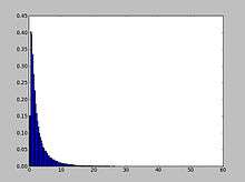
And to plot Wald distribution in Python using matplotlib and NumPy:

1 import matplotlib.pyplot as plt
2 import numpy as np
3 
4 h = plt.hist(np.random.wald(3, 2, 100000), bins=200, normed=True)
5 
6 plt.show()

Related distributions

• If $X\sim {\textrm {IG}}(\mu ,\lambda )\,$ then $kX\sim {\textrm {IG}}(k\mu ,k\lambda )\,$
• If $X_{i}\sim {\textrm {IG}}(\mu ,\lambda )\,$ then $\sum _{i=1}^{n}X_{i}\sim {\textrm {IG}}(n\mu ,n^{2}\lambda )\,$
• If $X_{i}\sim {\textrm {IG}}(\mu ,\lambda )\,$ for $i=1,\ldots ,n\,$ then ${\bar {X}}\sim {\textrm {IG}}(\mu ,n\lambda )\,$
• If $X_{i}\sim {\textrm {IG}}(\mu _{i},2\mu _{i}^{2})\,$ then $\sum _{{i=1}}^{{n}}X_{i}\sim {\textrm {IG}}\left(\sum _{{i=1}}^{n}\mu _{i},2{\left(\sum _{{i=1}}^{{n}}\mu _{i}\right)}^{2}\right)\,$

The convolution of an inverse Gaussian distribution (a Wald distribution) and an exponential (an ex-Wald distribution) is used as a model for response times in psychology,^[3] with visual search as one example.^[4]

History

This distribution appears to have been first derived by Schrödinger in 1915 as the time to first passage of a Brownian motion.^[5] The name inverse Gaussian was proposed by Tweedie in 1945.^[6] Wald re-derived this distribution in 1947 as the limiting form of a sample in a sequential probability ratio test. Tweedie investigated this distribution in 1957 and established some of its statistical properties.

Numeric computation and software

Despite the simple formula for the probability density function, numerical probability calculations for the inverse Gaussian distribution nevertheless require special care to achieve full machine accuracy in floating point arithmetic for all parameter values.^[7] Functions for the inverse Gaussian distribution are provided for the R programming language by the statmod package,^[8] available from the Comprehensive R Archive Network (CRAN).

See also

• Generalized inverse Gaussian distribution
• Tweedie distributions—The inverse Gaussian distribution is a member of the family of Tweedie exponential dispersion models
• Stopping time

References

1. Chhikara, Raj; Folks, Leroy (1989). The inverse Gaussian distribution: theory, methodology and applications. New York: Marcel Dekker. ISBN 0-8247-7997-5.
2. Michael, John R.; Schucany, William R.; Haas, Roy W. (May 1976). "Generating Random Variates Using Transformations with Multiple Roots". The American Statistician. American Statistical Association. 30 (2): 88–90. doi:10.2307/2683801. JSTOR 2683801.
3. Schwarz, W (2001). "The ex-Wald distribution as a descriptive model of response times". Behavior Research Methods, Instruments, and Computers. 33 (4): 457–69. PMID 11816448.
4. Palmer, E. M.; Horowitz, T. S.; Torralba, A.; Wolfe, J. M. (2011). "What are the shapes of response time distributions in visual search?". Journal of Experimental Psychology: Human Perception and Performance. 37: 58. doi:10.1037/a0020747.
5. Schrödinger, E. (1915). "Zur Theorie der Fall-und Steigversuche an Teilchen mit Brownscher Bewegung". Physikalische Zeitschrift. 16: 289–295.
6. Folks, J. L.; Chhikara, R. S. (1978). "The Inverse Gaussian Distribution and Its Statistical Application—A Review". Journal of the Royal Statistical Society. Series B (Methodological). 40 (3): 263–289. doi:10.2307/2984691 (inactive 2015-11-22). JSTOR 2984691.
7. Giner, Goknur; Smyth, Gordon (August 2016). "statmod: Probability Calculations for the Inverse Gaussian Distribution.". The R Journal. 8 (1): 339–351.
8. "statmod: Statistical Modeling".

Further reading

• Høyland, Arnljot; Rausand, Marvin (1994). System Reliability Theory. New York: Wiley. ISBN 0-471-59397-4.
• Seshadri, V. (1993). The Inverse Gaussian Distribution. Oxford University Press. ISBN 0-19-852243-6.

External links

• Inverse Gaussian Distribution in Wolfram website.