Markov random field
In the domain of physics and probability, a Markov random field (often abbreviated as MRF), Markov network or undirected graphical model is a set of random variables having a Markov property described by an undirected graph. In other words, a random field is said to be Markov random field if it satisfies Markov properties.
A Markov network or MRF is similar to a Bayesian network in its representation of dependencies; the differences being that Bayesian networks are directed and acyclic, whereas Markov networks are undirected and may be cyclic. Thus, a Markov network can represent certain dependencies that a Bayesian network cannot (such as cyclic dependencies); on the other hand, it can't represent certain dependencies that a Bayesian network can (such as induced dependencies). The underlying graph of a Markov random field may be finite or infinite.
When the joint probability density of the random variables is strictly positive, it is also referred to as a Gibbs random field, because, according to the Hammersley–Clifford theorem, it can then be represented by a Gibbs measure for an appropriate (locally defined) energy function. The prototypical Markov random field is the Ising model; indeed, the Markov random field was introduced as the general setting for the Ising model.[1] In the domain of artificial intelligence, a Markov random field is used to model various low- to mid-level tasks in image processing and computer vision.[2]
Definition
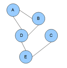
Given an undirected graph , a set of random variables indexed by form a Markov random field with respect to if they satisfy the local Markov properties:


- Pairwise Markov property: Any two non-adjacent variables are conditionally independent given all other variables:

- Local Markov property: A variable is conditionally independent of all other variables given its neighbors:
- where is the set of neighbors of , and is the closed neighbourhood of .


- Global Markov property: Any two subsets of variables are conditionally independent given a separating subset:
- where every path from a node in to a node in passes through .


The above three Markov properties are not equivalent: The Global Markov property is stronger than the Local Markov property, which in turn is stronger than the Pairwise one.
Clique factorization
As the Markov properties of an arbitrary probability distribution can be difficult to establish, a commonly used class of Markov random fields are those that can be factorized according to the cliques of the graph.
Given a set of random variables , let be the probability of a particular field configuration in . That is, is the probability of finding that the random variables take on the particular value . Because is a set, the probability of should be understood to be taken with respect to a joint distribution of the .


If this joint density can be factorized over the cliques of :

then forms a Markov random field with respect to . Here, is the set of cliques of . The definition is equivalent if only maximal cliques are used. The functions φC are sometimes referred to as factor potentials or clique potentials. Note, however, conflicting terminology is in use: the word potential is often applied to the logarithm of φC. This is because, in statistical mechanics, log(φC) has a direct interpretation as the potential energy of a configuration .


Although some MRFs do not factorize (a simple example can be constructed on a cycle of 4 nodes[3]), in certain cases they can be shown to be equivalent given certain conditions:
- if the density is positive (by the Hammersley–Clifford theorem),
- if the graph is chordal (by equivalence to a Bayesian network).
When such a factorization does exist, it is possible to construct a factor graph for the network.
Logistic model
Any Markov random field (with a strictly positive density) can be written as log-linear model with feature functions such that the full-joint distribution can be written as


where the notation

is simply a dot product over field configurations, and Z is the partition function:

Here, denotes the set of all possible assignments of values to all the network's random variables. Usually, the feature functions are defined such that they are indicators of the clique's configuration, i.e. if corresponds to the i-th possible configuration of the k-th clique and 0 otherwise. This model is equivalent to the clique factorization model given above, if is the cardinality of the clique, and the weight of a feature corresponds to the logarithm of the corresponding clique factor, i.e. , where is the i-th possible configuration of the k-th clique, i.e. the i-th value in the domain of the clique .


The probability P is often called the Gibbs measure. This expression of a Markov field as a logistic model is only possible if all clique factors are non-zero, i.e. if none of the elements of are assigned a probability of 0. This allows techniques from matrix algebra to be applied, e.g. that the trace of a matrix is log of the determinant, with the matrix representation of a graph arising from the graph's incidence matrix.
The importance of the partition function Z is that many concepts from statistical mechanics, such as entropy, directly generalize to the case of Markov networks, and an intuitive understanding can thereby be gained. In addition, the partition function allows variational methods to be applied to the solution of the problem: one can attach a driving force to one or more of the random variables, and explore the reaction of the network in response to this perturbation. Thus, for example, one may add a driving term Jv, for each vertex v of the graph, to the partition function to get:
![Z[J] = \sum_{x \in \mathcal{X}} \exp \left(\sum_{k} w_k^{\top} f_k(x_{ \{ k \} }) + \sum_v J_v x_v\right)](../I/m/773951a45d6bc3319ac9686893ec305b9be6a975.svg)
Formally differentiating with respect to Jv gives the expectation value of the random variable Xv associated with the vertex v:
![E[X_v] = \frac{1}{Z} \left.\frac{\partial Z[J]}{\partial J_v}\right|_{J_v=0}.](../I/m/6aefbf5571ffab813dc69951a5c713541ad58756.svg)
Correlation functions are computed likewise; the two-point correlation is:
![C[X_u, X_v] = \frac{1}{Z} \left.\frac{\partial^2 Z[J]}{\partial J_u \partial J_v}\right|_{J_u=0, J_v=0}.](../I/m/2cc174cc39c865e321b36f3ca9b02bfc76821570.svg)
Log-linear models are especially convenient for their interpretation. A log-linear model can provide a much more compact representation for many distributions, especially when variables have large domains. They are convenient too because their negative log likelihoods are convex. Unfortunately, though the likelihood of a logistic Markov network is convex, evaluating the likelihood or gradient of the likelihood of a model requires inference in the model, which is generally computationally infeasible (see 'Inference' below).
Examples
Gaussian
A multivariate normal distribution forms a Markov random field with respect to a graph if the missing edges correspond to zeros on the precision matrix (the inverse covariance matrix):

such that

Inference
As in a Bayesian network, one may calculate the conditional distribution of a set of nodes given values to another set of nodes in the Markov random field by summing over all possible assignments to ; this is called exact inference. However, exact inference is a #P-complete problem, and thus computationally intractable in the general case. Approximation techniques such as Markov chain Monte Carlo and loopy belief propagation are often more feasible in practice. Some particular subclasses of MRFs, such as trees (see Chow–Liu tree), have polynomial-time inference algorithms; discovering such subclasses is an active research topic. There are also subclasses of MRFs that permit efficient MAP, or most likely assignment, inference; examples of these include associative networks.[5][6] Another interesting sub-class is the one of decomposable models (when the graph is chordal): having a closed-form for the MLE, it is possible to discover a consistent structure for hundreds of variables.[7]


Conditional random fields
One notable variant of a Markov random field is a conditional random field, in which each random variable may also be conditioned upon a set of global observations . In this model, each function is a mapping from all assignments to both the clique k and the observations to the nonnegative real numbers. This form of the Markov network may be more appropriate for producing discriminative classifiers, which do not model the distribution over the observations. CRFs were proposed by John D. Lafferty, Andrew McCallum and Fernando C.N. Pereira in 2001.[8]


Varied applications
Markov random fields find application in a variety of fields, ranging from computer graphics to computer vision and machine learning.[9] MRFs are used in image processing to generate textures as they can be used to generate flexible and stochastic image models. In image modelling, the task is to find a suitable intensity distribution of a given image, where suitability depends on the kind of task and MRFs are flexible enough to be used for image and texture synthesis, image compression and restoration, image segmentation, surface reconstruction, image registration, texture synthesis, super-resolution, stereo matching and information retrieval. They can be used to solve various computer vision problems which can be posed as energy minimization problems or problems where different regions have to be distinguished using a set of discriminating features, within a Markov random field framework, to predict the category of the region.[10] Markov random fields were a generalization over the Ising model and have, since then, been used widely in combinatorial optimizations and networks.
See also
- Constraint Composite Graph
- Graphical model
- Hammersley–Clifford theorem
- Hopfield network
- Interacting particle system
- Ising model
- Log-linear analysis
- Markov chain
- Markov logic network
- Maximum entropy method
- Probabilistic cellular automata
References
- ↑ Kindermann, Ross; Snell, J. Laurie (1980). Markov Random Fields and Their Applications (PDF). American Mathematical Society. ISBN 0-8218-5001-6. MR 0620955.
- ↑ Li, S. Z. (2009). Markov Random Field Modeling in Image Analysis. Springer.
- ↑ Moussouris, John (1974). "Gibbs and Markov random systems with constraints". Journal of Statistical Physics. 10 (1): 11–33. doi:10.1007/BF01011714. MR 0432132.
- ↑ Rue, Håvard; Held, Leonhard (2005). Gaussian Markov random fields: theory and applications. CRC Press. ISBN 1-58488-432-0.
- ↑ Taskar, Benjamin; Chatalbashev, Vassil; Koller, Daphne (2004), "Learning associative Markov networks", in Brodley, Carla E., Proceedings of the Twenty-first International Conference on Machine Learning (ICML 2004), Banff, Alberta, Canada, July 4-8, 2004, ACM International Conference Proceeding Series, 69, Association for Computing Machinery, doi:10.1145/1015330.1015444.
- ↑ Duchi, John C.; Tarlow, Daniel; Elidan, Gal; Koller, Daphne (2006), "Using Combinatorial Optimization within Max-Product Belief Propagation", in Schölkopf, Bernhard; Platt, John C.; Hoffman, Thomas, Proceedings of the Twentieth Annual Conference on Neural Information Processing Systems, Vancouver, British Columbia, Canada, December 4-7, 2006, Advances in Neural Information Processing Systems, 19, MIT Press, pp. 369–376.
- ↑ Petitjean, F.; Webb, G.I.; Nicholson, A.E. (2013). Scaling log-linear analysis to high-dimensional data (PDF). International Conference on Data Mining. Dallas, TX, USA: IEEE.
- ↑ "Two classic paper prizes for papers that appeared at ICML 2013". ICML. 2013. Retrieved 15 December 2014.
- ↑ Kindermann & Snell, Ross & Laurie (1980). Markov Random Fields and their Applications. Rhode Island: American Mathematical Society. ISBN 0-8218-5001-6.
- ↑ Zhang & Zakhor, Richard & Avideh (2014). "Automatic Identification of Window Regions on Indoor Point Clouds Using LiDAR and Cameras". VIP Lab Publications.