Wave function
A wave function in quantum mechanics is a description of the quantum state of a system. The wave function is a complex-valued probability amplitude, and the probabilities for the possible results of measurements made on the system can be derived from it. The most common symbols for a wave function are the Greek letters ψ or Ψ (lower-case and capital psi).
The wave function is a function of the degrees of freedom corresponding to some maximal set of commuting observables. Once such a representation is chosen, the wave function can be derived from the quantum state.
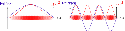
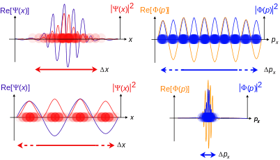
For a given system, the choice of which commuting degrees of freedom to use is not unique, and correspondingly the domain of the wave function is not unique. For instance it may be taken to be a function of all the position coordinates of the particles over position space, or the momenta of all the particles over momentum space, the two are related by a Fourier transform. Some particles, like electrons and photons, have nonzero spin, and the wave function for such particles includes spin as an intrinsic, discrete degree of freedom. Other discrete variables can also be included, such as isospin. When a system has internal degrees of freedom, the wave function at each point in the continuous degrees of freedom (e.g. a point in space) assigns a complex number for each possible value of the discrete degrees of freedom (e.g. z-component of spin). These values are often displayed in a column matrix (e.g. a 2 × 1 column vector for a non-relativistic electron with spin 1⁄2).
According to the superposition principle of quantum mechanics, wave functions can be added together and multiplied by complex numbers to form new wave functions and form a Hilbert space. The inner product between two wave functions is a measure of the overlap between the corresponding physical states and is used in the foundational probabilistic interpretation of quantum mechanics, the Born rule, relating transition probabilities to inner products. The Schrödinger equation determines how wave functions evolve over time. A wave function behaves qualitatively like other waves, such as water waves or waves on a string, because the Schrödinger equation is mathematically a type of wave equation. This explains the name "wave function", and gives rise to wave–particle duality. However, the wave function in quantum mechanics describes a kind of physical phenomenon, still open to different interpretations, which fundamentally differs from that of classic mechanical waves.[1][2][3][4][5][6][7]
In Born's statistical interpretation in non-relativistic quantum mechanics,[8][9][10] the squared modulus of the wave function, | ψ |2, is a real number interpreted as the probability density of measuring a particle's being detected at a given place, or having a given momentum, at a given time, and possibly having definite values for discrete degrees of freedom. The integral of this quantity, over all the system's degrees of freedom, must be 1 in accordance with the probability interpretation, this general requirement a wave function must satisfy is called the normalization condition. Since the wave function is complex valued, only its relative phase and relative magnitude can be measured. Its value does not in isolation tell anything about the magnitudes or directions of measurable observables; one has to apply quantum operators, whose eigenvalues correspond to sets of possible results of measurements, to the wave function ψ and calculate the statistical distributions for measurable quantities.
Historical background

In 1905 Einstein postulated the proportionality between the frequency of a photon and its energy, E = hf,[11] and in 1916 the corresponding relation between photon momentum and wavelength, λ = h/p.[12] In 1923, De Broglie was the first to suggest that the relation λ = h/p, now called the De Broglie relation, holds for massive particles, the chief clue being Lorentz invariance,[13] and this can be viewed as the starting point for the modern development of quantum mechanics. The equations represent wave–particle duality for both massless and massive particles.
In the 1920s and 1930s, quantum mechanics was developed using calculus and linear algebra. Those who used the techniques of calculus included Louis de Broglie, Erwin Schrödinger, and others, developing "wave mechanics". Those who applied the methods of linear algebra included Werner Heisenberg, Max Born, and others, developing "matrix mechanics". Schrödinger subsequently showed that the two approaches were equivalent.[14]
In 1926, Schrödinger published the famous wave equation now named after him, indeed the Schrödinger equation, based on classical Conservation of energy using quantum operators and the de Broglie relations such that the solutions of the equation are the wave functions for the quantum system.[15] However, no one was clear on how to interpret it.[16] At first, Schrödinger and others thought that wave functions represent particles that are spread out with most of the particle being where the wave function is large.[17] This was shown to be incompatible with how elastic scattering of a wave packet representing a particle off a target appears; it spreads out in all directions.[8] While a scattered particle may scatter in any direction, it does not break up and take off in all directions. In 1926, Born provided the perspective of probability amplitude.[8][9][18] This relates calculations of quantum mechanics directly to probabilistic experimental observations. It is accepted as part of the Copenhagen interpretation of quantum mechanics. There are many other interpretations of quantum mechanics. In 1927, Hartree and Fock made the first step in an attempt to solve the N-body wave function, and developed the self-consistency cycle: an iterative algorithm to approximate the solution. Now it is also known as the Hartree–Fock method.[19] The Slater determinant and permanent (of a matrix) was part of the method, provided by John C. Slater.
Schrödinger did encounter an equation for the wave function that satisfied relativistic energy conservation before he published the non-relativistic one, but discarded it as it predicted negative probabilities and negative energies. In 1927, Klein, Gordon and Fock also found it, but incorporated the electromagnetic interaction and proved that it was Lorentz invariant. De Broglie also arrived at the same equation in 1928. This relativistic wave equation is now most commonly known as the Klein–Gordon equation.[20]
In 1927, Pauli phenomenologically found a non-relativistic equation to describe spin-1/2 particles in electromagnetic fields, now called the Pauli equation.[21] Pauli found the wave function was not described by a single complex function of space and time, but needed two complex numbers, which respectively correspond to the spin +1/2 and −1/2 states of the fermion. Soon after in 1928, Dirac found an equation from the first successful unification of special relativity and quantum mechanics applied to the electron, now called the Dirac equation. In this, the wave function is a spinor represented by four complex-valued components:[19] two for the electron and two for the electron's antiparticle, the positron. In the non-relativistic limit, the Dirac wave function resembles the Pauli wave function for the electron. Later, other relativistic wave equations were found.
Wave functions and wave equations in modern theories
All these wave equations are of enduring importance. The Schrödinger equation and the Pauli equation are under many circumstances excellent approximations of the relativistic variants. They are considerably easier to solve in practical problems than the relativistic counterparts.
The Klein-Gordon equation and the Dirac equation, while being relativistic, do not represent full reconciliation of quantum mechanics and special relativity. The branch of quantum mechanics where these equations are studied the same way as the Schrödinger equation, often called relativistic quantum mechanics, while very successful, has its limitations (see e.g. Lamb shift) and conceptual problems (see e.g. Dirac sea).
Relativity makes it inevitable that the number of particles in a system is not constant. For full reconciliation, quantum field theory is needed.[22] In this theory, the wave equations and the wave functions have their place, but in a somewhat different guise. The main objects of interest are not the wave functions, but rather operators, so called field operators (or just fields where "operator" is understood) on the Hilbert space of states (to be described next section). It turns out that the original relativistic wave equations and their solutions are still needed to build the Hilbert space. Moreover, the free fields operators, i.e. when interactions are assumed not to exist, turn out to (formally) satisfy the same equation as do the fields (wave functions) in many cases.
Thus the Klein-Gordon equation (spin 0) and the Dirac equation (spin 1⁄2) in this guise remain in the theory. Higher spin analogues include the Proca equation (spin 1), Rarita–Schwinger equation (spin 3⁄2), and, more generally, the Bargmann–Wigner equations. For massless free fields two examples are the free field Maxwell equation (spin 1) and the free field Einstein equation (spin 2) for the field operators.[23] All of them are essentially a direct consequence of the requirement of Lorentz invariance. Their solutions must transform under Lorentz transformation in a prescribed way, i.e. under a particular representation of the Lorentz group and that together with few other reasonable demands, e.g. the cluster decomposition principle,[24] with implications for causality is enough to fix the equations.
It should be emphasized that this applies to free field equations; interactions are not included. If a Lagrangian density (including interactions) is available, then the Lagrangian formalism will yield an equation of motion at the classical level. This equation may be very complex and not amenable to solution. Any solution would refer to a fixed number of particles and would not account for the term "interaction" as referred to in these theories, which involves the creation and annihilation of particles and not external potentials as in ordinary "first quantized" quantum theory.
In string theory, the situation remains analogous. For instance, a wave function in momentum space has the role of Fourier expansion coefficient in a general state of a particle (string) with momentum that is not sharply defined.[25]
Definition (one spinless particle in 1d)
For now, consider the simple case of a non-relativistic single particle, without spin, in one spatial dimension. More general cases are discussed below.
Position-space wave functions
The state of such a particle is completely described by its wave function,

where x is position and t is time. This is a complex-valued function of two real variables x and t.
For one spinless particle in 1d, if the wave function is interpreted as a probability amplitude, the square modulus of the wave function, the positive real number

is interpreted as the probability density that the particle is at x. The asterisk indicates the complex conjugate. If the particle's position is measured, its location cannot be determined from the wave function, but is described by a probability distribution. The probability that its position x will be in the interval a ≤ x ≤ b is the integral of the density over this interval:

where t is the time at which the particle was measured. This leads to the normalization condition:

because if the particle is measured, there is 100% probability that it will be somewhere.
For a given system, the set of all possible normalizable wave functions (at any given time) forms an abstract mathematical vector space, meaning that it is possible to add together different wave functions, and multiply wave functions by complex numbers (see vector space for details). Technically, because of the normalization condition, wave functions form a projective space rather than an ordinary vector space. This vector space is infinite-dimensional, because there is no finite set of functions which can be added together in various combinations to create every possible function. Also, it is a Hilbert space, because the inner product of two wave functions Ψ1 and Ψ2 can be defined as the complex number (at time t)[nb 1]

More details are given below. Although the inner product of two wave functions is a complex number, the inner product of a wave function Ψ with itself,

is always a positive real number. The number ||Ψ|| (not ||Ψ||2) is called the norm of the wave function Ψ, and is not the same as the modulus |Ψ|.
If (Ψ, Ψ) = 1, then Ψ is normalized. If Ψ is not normalized, then dividing by its norm gives the normalized function Ψ/||Ψ||. Two wave functions Ψ1 and Ψ2 are orthogonal if (Ψ1, Ψ2) = 0. If they are normalized and orthogonal, they are orthonormal. Orthogonality (hence also orthonormality) of wave functions is not a necessary condition wave functions must satisfy, but is instructive to consider since this guarantees linear independence of the functions. In a linear combination of orthogonal wave functions Ψn we have,

If the wave functions Ψn were nonorthogonal, the coefficients would be less simple to obtain.
In the Copenhagen interpretation, the modulus squared of the inner product (a complex number) gives a real number

which, assuming both wave functions are normalized, is interpreted as the probability of the wave function Ψ2 "collapsing" to the new wave function Ψ1 upon measurement of an observable, whose eigenvalues are the possible results of the measurement, with Ψ1 being an eigenvector of the resulting eigenvalue. This is the Born rule,[8] and is one of the fundamental postulates of quantum mechanics.
At a particular instant of time, all values of the wave function Ψ(x, t) are components of a vector. There are uncountably infinitely many of them and integration is used in place of summation. In Bra–ket notation, this vector is written

and is referred to as a "quantum state vector", or simply "quantum state".There are several advantages to understanding wave functions as representing elements of an abstract vector space:
- All the powerful tools of linear algebra can be used to manipulate and understand wave functions. For example:
- Linear algebra explains how a vector space can be given a basis, and then any vector in the vector space can be expressed in this basis. This explains the relationship between a wave function in position space and a wave function in momentum space, and suggests that there are other possibilities too.
- Bra–ket notation can be used to manipulate wave functions.
- The idea that quantum states are vectors in an abstract vector space is completely general in all aspects of quantum mechanics and quantum field theory, whereas the idea that quantum states are complex-valued "wave" functions of space is only true in certain situations.
The time parameter is often suppressed, and will be in the following. The x coordinate is a continuous index. The |x⟩ are the basis vectors, which are orthonormal so their inner product is a delta function;

thus

and

which illuminates the identity operator

Finding the identity operator in a basis allows the abstract state to be expressed explicitly in a basis, and more (the inner product between two state vectors, and other operators for observables, can be expressed in the basis).
Momentum-space wave functions
The particle also has a wave function in momentum space:

where p is the momentum in one dimension, which can be any value from −∞ to +∞, and t is time.
Analogous to the position case, the inner product of two wave functions Φ1(p, t) and Φ2(p, t) can be defined as:

One particular solution to the time-independent Schrödinger equation is

a plane wave, which can be used in the description of a particle with momentum exactly p, since it is an eigenfunction of the momentum operator. These functions are not normalizable to unity (they aren't square-integrable), so they are not really elements of physical Hilbert space. The set

forms what is called the momentum basis. This "basis" is not a basis in the usual mathematical sense. For one thing, since the functions aren't normalizable, they are instead normalized to a delta function,

For another thing, though they are linearly independent, there are too many of them (they form an uncountable set) for a basis for physical Hilbert space. They can still be used to express all functions in it using Fourier transforms as described next.
Relations between position and momentum representations
The x and p representations are

Now take the projection of the state Ψ onto eigenfunctions of momentum using the last expression in the two equations,[26]

Then utilizing the known expression for suitably normalized eigenstates of momentum in the position representation solutions of the free Schrödinger equation

one obtains

Likewise, using eigenfunctions of position,

The position-space and momentum-space wave functions are thus found to be Fourier transforms of each other.[27] The two wave functions contain the same information, and either one alone is sufficient to calculate any property of the particle. As representatives of elements of abstract physical Hilbert space, whose elements are the possible states of the system under consideration, they represent the same state vector, hence identical physical states, but they are not generally equal when viewed as square-integrable functions.
In practice, the position-space wave function is used much more often than the momentum-space wave function. The potential entering the relevant equation (Schrödinger, Dirac, etc.) determines in which basis the description is easiest. For the harmonic oscillator, x and p enter symmetrically, so there it doesn't matter which description one uses. The same equation (modulo constants) results. From this follows, with a little bit of afterthought, a factoid: The solutions to the wave equation of the harmonic oscillator are eigenfunctions of the Fourier transform in L2.[nb 2]
Definitions (other cases)
Following are the general forms of the wave function for systems in higher dimensions and more particles, as well as including other degrees of freedom than position coordinates or momentum components.
One-particle states in 3d position space
The position-space wave function of a single particle without spin in three spatial dimensions is similar to the case of one spatial dimension above:

where r is the position vector in three-dimensional space, and t is time. As always Ψ(r, t) is a complex-valued function of real variables. As a single vector in Dirac notation

All the previous remarks on inner products, momentum space wave functions, Fourier transforms, and so on extend to higher dimensions.
For a particle with spin, ignoring the position degrees of freedom, the wave function is a function of spin only (time is a parameter);

where sz is the spin projection quantum number along the z axis. (The z axis is an arbitrary choice; other axes can be used instead if the wave function is transformed appropriately, see below.) The sz parameter, unlike r and t, is a discrete variable. For example, for a spin-1/2 particle, sz can only be +1/2 or −1/2, and not any other value. (In general, for spin s, sz can be s, s − 1, ... , −s + 1, −s). Inserting each quantum number gives a complex valued function of space and time, there are 2s + 1 of them. These can be arranged into a column vector[nb 3]

In bra ket notation, these easily arrange into the components of a vector[nb 4]

The entire vector ξ is a solution of the Schrödinger equation (with a suitable Hamiltonian), which unfolds to a coupled system of 2s + 1 ordinary differential equations with solutions ξ(s, t), ξ(s − 1, t), ..., ξ(−s, t). The term "spin function" instead of "wave function" is used by some authors. This contrasts the solutions to position space wave functions, the position coordinates being continuous degrees of freedom, because then the Schrödinger equation does take the form of a wave equation.
More generally, for a particle in 3d with any spin, the wave function can be written in "position–spin space" as:

and these can also be arranged into a column vector

in which the spin dependence is placed in indexing the entries, and the wave function is a complex vector-valued function of space and time only.
All values of the wave function, not only for discrete but continuous variables also, collect into a single vector

For a single particle, the tensor product ⊗ of its position state vector |ψ⟩ and spin state vector |ξ⟩ gives the composite position-spin state vector

with the identifications


The tensor product factorization is only possible if the orbital and spin angular momenta of the particle are separable in the Hamiltonian operator underlying the system's dynamics (in other words, the Hamiltonian can be split into the sum of orbital and spin terms[28]). The time dependence can be placed in either factor, and time evolution of each can be studied separately. The factorization is not possible for those interactions where an external field or any space-dependent quantity couples to the spin; examples include a particle in a magnetic field, and spin-orbit coupling.
The preceding discussion is not limited to spin as a discrete variable, the total angular momentum J may also be used.[29] Other discrete degrees of freedom, like isospin, can expressed similarly to the case of spin above.
Many particle states in 3d position space
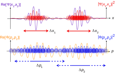
If there are many particles, in general there is only one wave function, not a separate wave function for each particle. The fact that one wave function describes many particles is what makes quantum entanglement and the EPR paradox possible. The position-space wave function for N particles is written:[19]

where ri is the position of the ith particle in three-dimensional space, and t is time. Altogether, this is a complex-valued function of 3N + 1 real variables.
In quantum mechanics there is a fundamental distinction between identical particles and distinguishable particles. For example, any two electrons are identical and fundamentally indistinguishable from each other; the laws of physics make it impossible to "stamp an identification number" on a certain electron to keep track of it.[27] This translates to a requirement on the wave function for a system of identical particles:

where the + sign occurs if the particles are all bosons and − sign if they are all fermions. In other words, the wave function is either totally symmetric in the positions of bosons, or totally antisymmetric in the positions of fermions.[30] The physical interchange of particles corresponds to mathematically switching arguments in the wave function. The antisymmetry feature of fermionic wave functions leads to the Pauli principle. Generally, bosonic and fermionic symmetry requirements are the manifestation of particle statistics and are present in other quantum state formalisms.
For N distinguishable particles (no two being identical, i.e. no two having the same set of quantum numbers), there is no requirement for the wave function to be either symmetric or antisymmetric.
For a collection of particles, some identical with coordinates r1, r2, ... and others distinguishable x1, x2, ... (not identical with each other, and not identical to the aforementioned identical particles), the wave function is symmetric or antisymmetric in the identical particle coordinates ri only:

Again, there is no symmetry requirement for the distinguishable particle coordinates xi.
The wave function for N particles each with spin is the complex-valued function

Accumulating all these components into a single vector,

For identical particles, symmetry requirements apply to both position and spin arguments of the wave function so it has the overall correct symmetry.
The formulae for the inner products are integrals over all coordinates or momenta and sums over all spin quantum numbers. For the general case of N particles with spin in 3d,

this is altogether N three-dimensional volume integrals and N sums over the spins. The differential volume elements d3ri are also written "dVi" or "dxi dyi dzi".
The multidimensional Fourier transforms of the position or position–spin space wave functions yields momentum or momentum–spin space wave functions.
Probability interpretation
For the general case of N particles with spin in 3d, if Ψ is interpreted as a probability amplitude, the probability density is

and the probability that particle 1 is in region R1 with spin sz1 = m1 and particle 2 is in region R2 with spin sz2 = m2 etc. at time t is the integral of the probability density over these regions and evaluated at these spin numbers:

Time dependence
For systems in time-independent potentials, the wave function can always be written as a function of the degrees of freedom multiplied by a time-dependent phase factor, the form of which is given by the Schrödinger equation. For N particles, considering their positions only and suppressing other degrees of freedom,

where E is the energy eigenvalue of the system corresponding to the eigenstate Ψ. Wave functions of this form are called stationary states.
The time dependence of the quantum state and the operators can be placed according to unitary transformations on the operators and states. For any quantum state |Ψ⟩ and operator O, in the Schrödinger picture |Ψ(t)⟩ changes with time according to the Schrödinger equation while O is constant. In the Heisenberg picture it is the other way round, |Ψ⟩ is constant while O(t) evolves with time according to the Heisenberg equation of motion. The Dirac (or interaction) picture is intermediate, time dependence is places in both operators and states which evolve according to equations of motion. It is useful primarily in computing S-matrix elements.[31]
Non-relativistic examples
The following are solutions to the Schrödinger equation for one nonrelativistic spinless particle.
Particle in a box
A simple model is the particle in a box, a particle is restricted to a 1D region between x = 0 and x = L subject to a potential

has the normalized wave function

Finite potential barrier
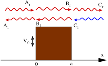
One of most prominent features of the wave mechanics is a possibility for a particle to reach a location with a prohibitive (in classical mechanics) force potential. A common model is the "potential barrier", the one-dimensional case has the potential

and the steady-state solutions to the wave equation have the form (for some constants k, κ)

Note that these wave functions are not normalized; see scattering theory for discussion.
The standard interpretation of this is as a stream of particles being fired at the step from the left (the direction of negative x): setting Ar = 1 corresponds to firing particles singly; the terms containing Ar and Cr signify motion to the right, while Al and Cl – to the left. Under this beam interpretation, put Cl = 0 since no particles are coming from the right. By applying the continuity of wave functions and their derivatives at the boundaries, it is hence possible to determine the constants above.
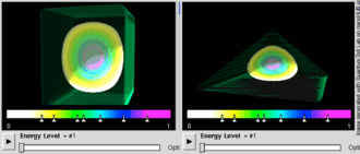
In a semiconductor crystallite whose radius is smaller than the size of its exciton Bohr radius, the excitons are squeezed, leading to quantum confinement. The energy levels can then be modeled using the particle in a box model in which the energy of different states is dependent on the length of the box.
Quantum harmonic oscillator
The wave functions for the quantum harmonic oscillator can be expressed in terms of Hermite polynomials Hn, they are

where n = 0,1,2,....
Hydrogen atom
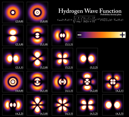
The wave functions of an electron in a Hydrogen atom are expressed in terms of spherical harmonics and generalized Laguerre polynomials (these are defined differently by different authors—see main article on them and the hydrogen atom).
It is convenient to use spherical coordinates, and the wavefunction can be separated into functions of each coordinate,[32]

where R are radial functions and Ym
ℓ(θ, φ) are spherical harmonics of degree ℓ and order m. This is the only atom for which the Schrödinger equation has been solved for exactly. Multi-electron atoms require approximative methods. The family of solutions are:[33]
![{\displaystyle \Psi _{n\ell m}(r,\theta ,\phi )={\sqrt {{\left({\frac {2}{na_{0}}}\right)}^{3}{\frac {(n-\ell -1)!}{2n[(n+\ell )!]}}}}e^{-r/na_{0}}\left({\frac {2r}{na_{0}}}\right)^{\ell }L_{n-\ell -1}^{2\ell +1}\left({\frac {2r}{na_{0}}}\right)\cdot Y_{\ell }^{m}(\theta ,\phi )}](../I/m/79cdce8d7174c4b860efa65d1422b5550537284f.svg)
where a0 = 4πε0ħ2/mee2 is the Bohr radius,
L2ℓ + 1
n − ℓ − 1 are the generalized Laguerre polynomials of degree n − ℓ − 1, n = 1, 2, ... is the principal quantum number, ℓ = 1, 2, ... n − 1 the azimuthal quantum number, m = −ℓ, −ℓ + 1, ..., ℓ − 1, ℓ the magnetic quantum number. Hydrogen-like atoms have very similar solutions.
This solution does not take into account the spin of the electron.
In the figure of the hydrogen orbitals, the 19 sub-images are images of wave functions in position space (their norm squared). The wave functions each represent the abstract state characterized by the triple of quantum numbers (n, l, m), in the lower right of each image. These are the principal quantum number, the orbital angular momentum quantum number and the magnetic quantum number. Together with one spin-projection quantum number of the electron, this is a complete set of observables.
The figure can serve to illustrate some further properties of the function spaces of wave functions.
- In this case, the wave functions are square integrable. One can initially take the function space as the space of square integrable functions, usually denoted L2.
- The displayed functions are solutions to the Schrödinger equation. Obviously, not every function in L2 satisfies the Schrödinger equation for the hydrogen atom. The function space is thus a subspace of L2.
- The displayed functions form part of a basis for the function space. To each triple (n, l, m), there corresponds a basis wave function. If spin is taken into account, there are two basis functions for each triple. The function space thus has a countable basis.
- The basis functions are mutually orthonormal.
Wave functions and function spaces
The concept of function spaces enters naturally in the discussion about wave functions. A function space is a set of functions, usually with some defining requirements on the functions (in the present case that they are square integrable), sometimes with an algebraic structure on the set (in the present case a vector space structure with an inner product), together with a topology on the set. The latter will sparsely be used here, it is only needed to obtain a precise definition of what it means for a subset of a function space to be closed. It will be concluded below that the function space of wave functions is a Hilbert space. This observation is the foundation of the predominant mathematical formulation of quantum mechanics.
Vector space structure
A wave function is an element of a function space partly characterized by the following concrete and abstract descriptions.
- The Schrödinger equation is linear. This means that the solutions to it, wave functions, can be added and multiplied by scalars to form a new solution. The set of solutions to the Schrödinger equation is a vector space.
- The superposition principle of quantum mechanics. If Ψ and Φ are two states in the abstract space of states of a quantum mechanical system, and a and b are any two complex numbers, then aΨ + bΦ is a valid state as well. (Whether the null vector counts as a valid state ("no system present") is a matter of definition. The null vector does not at any rate describe the vacuum state in quantum field theory.) The set of allowable states is a vector space.
This similarity is of course not accidental. There are also a distinctions between the spaces to keep in mind.
Representations
Basic states are characterized by a set of quantum numbers. This is a set of eigenvalues of a maximal set of commuting observables. Physical observables are represented by linear operators, also called observables, on the vectors space. Maximality means that there can be added to the set no further algebraically independent observables that commute with the ones already present. A choice of such a set may be called a choice of representation.
- It is a postulate of quantum mechanics that a physically observable quantity of a system, such as position, momentum, or spin, is represented by a linear Hermitian operator on the state space. The possible outcomes of measurement of the quantity are the eigenvalues of the operator.[17] At a deeper level, most observables, perhaps all, arise as generators of symmetries.[17][34][nb 5]
- The physical interpretation is that such a set represents what can – in theory – be simultaneously be measured with arbitrary precision. The Heisenberg uncertainty relation prohibits simultaneous exact measurements of two non-commuting observables.
- The set is non-unique. It may for a one-particle system, for example, be position and spin z-projection, (x, Sz), or it may be momentum and spin y-projection, (p, Sy). In this case, the operator corresponding to position (a multiplication operator in the position representation) and the operator corresponding to momentum (a differential operator in the position the position representation) do not commute.
- Once a representation is chosen, there is still arbitrariness. It remains to choose a coordinate system. This may, for example, correspond to a choice of x, y- and z-axis, or a choice of curvilinear coordinates as exemplified by the spherical coordinates used for the Hydrogen atomic wave functions. This final choice also fixes a basis in abstract Hilbert space. The basic states are labeled by the quantum numbers corresponding to the maximal set of commuting observables and an appropriate coordinate system.[nb 6]
The abstract states are "abstract" only in that an arbitrary choice necessary for a particular explicit description of it is not given. This is the same as saying that no choice of maximal set of commuting observables has been given. This is analogous to a vector space without a specified basis. Wave functions corresponding to a state are accordingly not unique. This non-uniqueness reflects the non-uniqueness in the choice of a maximal set of commuting observables. For one spin particle in one dimension, to a particular state there corresponds two wave functions, Ψ(x, Sz) and Ψ(p, Sy), both describing the same state.
- For each choice of maximal commuting sets of observables for the abstract state space, there is a corresponding representation that is associated to a function space of wave functions.
- Between all these different function spaces and the abstract state space, there are one-to-one correspondences (here disregarding normalization and unobservable phase factors), the common denominator here being a particular abstract state. The relationship between the momentum and position space wave functions, for instance, describing the same state is the Fourier transform.
Each choice of representation should be thought of as specifying a unique function space in which wave functions corresponding to that choice of representation lives. This distinction is best kept, even if one could argue that two such function spaces are mathematically equal, e.g. being the set of square integrable functions. One can then think of the function spaces as two distinct copies of that set.
Inner product
There is additional algebraic structure on the vector spaces of wave functions and the abstract state space.
- Physically, different wave functions are interpreted to overlap to some degree. A system in a state Ψ that does not overlap with a state Φ cannot be found to be in the state Φ upon measurement. But if Φ1, Φ2, ... overlap Ψ to some degree, there is a chance that measurement of a system described by Ψ will be found un states Φ1, Φ2, ... . Also selection rules are observed apply. These are usually formulated in the preservation of some quantum numbers. This means that certain processes allowable from some perspectives (e.g. energy and momentum conservation) do not occur because the initial and final total wave functions don't overlap.
- Mathematically, it turns out that solutions to the Schrödinger equation for particular potentials are orthogonal in some manner, this is usually described by an integral
- where m, n are (sets of) indices (quantum numbers) labeling different solutions, the strictly positive function w is called a weight function, and δmn is the Kronecker delta. The integration is taken over all of the relevant space.

This motivates the introduction of an inner product on the vector space of abstract quantum states, compatible with the mathematical observations of above when passing to a representation. It is denoted (Ψ, Φ), or in the Bra–ket notation ⟨Ψ|Φ⟩. It yields a complex number. With the inner product, the function space is an inner product space. The explicit appearance of the inner product (usually an integral or a sum of integrals) depends on the choice of representation, but the complex number (Ψ, Φ) does not. Much of the physical interpretation of quantum mechanics stems from the Born rule. It states that the probability p of finding upon measurement the state Φ given the system is in the state Ψ is

where Φ and Ψ are assumed normalized. Consider a scattering experiment. In quantum field theory, if Φout describes a state in the "distant future" (an "out state") after interactions between scattering particles have ceased, and Ψin an "in state" in the "distant past", then the quantities (Φout, Ψin), with Φout and Ψin varying over a complete set of in states and out states respectively, is called the S-matrix or scattering matrix. Knowledge of it is, effectively, having solved the theory at hand, at least as far as predictions go. Measurable quantities such as decay rates and scattering cross sections are calculable from the S-matric.[35]
Hilbert space
The above observations encapsulate the essence of the function spaces of which wave functions are elements. However the description is not yet complete. There is a further technical requirement on the function space, that of completeness, that allows one to take limits of sequences in the function space, and be ensured that, if the limit exists, it is an element of the function space. A complete inner product space is called a Hilbert space. The property of completeness is crucial in advanced treatments and applications of quantum mechanics. For instance, the existence of projection operators or orthogonal projections relies on the completeness of the space.[36] These projection operators, in turn, are essential for the statement and proof of many useful theorems, e.g. the spectral theorem. It is not very important in the in introductory quantum mechanics, and technical details and links may be found in footnotes like the one that follows.[nb 7] The space L2 is a Hilbert space, with inner product presented later. The function space of the example of the figure is a subspace of L2. A subspace of a Hilbert space is a Hilbert space if it is closed.
In summary, the set of all possible normalizable wave functions for a system with a particular choice of basis, together with the null vector, constitute a Hilbert space.
Not all functions of interest are elements of some Hilbert space, say L2. The most glaring example is the set of functions e 2πip · x⁄h. These are plane wave solutions of the Schrödinger equation for a free particle, but are not normalizable, hence not in L2. But they are nonetheless fundamental for the description. One can, using them, express functions that are normalizable using wave packets. They are, in a sense, a basis (but not a Hilbert space basis, nor a Hamel basis) in which wave functions of interest can be expressed. There is also the artifact "normalization to a delta function" that is frequently employed for notational convenience, see further down. The delta functions themselves aren't square integrable either.
The above description of the function space containing the wave functions is mostly mathematically motivated. The function spaces are, due to completeness, very large in a certain sense. Not all functions are realistic descriptions of any physical system. For instance, in the function space L2 one can find the function that takes on the value 0 for all rational numbers and -i for the irrationals in the interval [0, 1]. This is square integrable,[nb 8] but can hardly represent a physical state.
Common Hilbert spaces
While the space of solutions as a whole is a Hilbert space there are many other Hilbert spaces that commonly occur as ingredients.
- Square integrable complex valued functions on the interval [0, 2π]. The set {eint/2π, n ∈ ℤ} is a Hilbert space basis, i.e. a maximal orthonormal set.
- The Fourier transform takes functions in the above space to elements of l2(ℤ), the space of square summable functions ℤ → ℂ. The latter space is a Hilbert space and the Fourier transform is an isomorphism of Hilbert spaces.[nb 9] Its basis is {ei, i ∈ ℤ} with ei(j) = δij, i, j ∈ ℤ.
- The most basic example of spanning polynomials is in the space of square integrable functions on the interval [–1, 1] for which the Legendre polynomials is a Hilbert space basis (complete orthonormal set).
- The square integrable functions on the unit sphere S2 is a Hilbert space. The basis functions in this case are the spherical harmonics. The Legendre polynomials are ingredients in the spherical harmonics. Most problems with rotational symmetry will have "the same" (known) solution with respect to that symmetry, so the original problem is reduced to a problem of lower dimensionality.
- The associated Laguerre polynomials appear in the hydrogenic wave function problem after factoring out the spherical harmonics. These span the Hilbert space of square integrable functions on the semi-infinite interval [0, ∞).
More generally, one may consider a unified treatment of all second order polynomial solutions to the Sturm–Liouville equations in the setting of Hilbert space. These include the Legendre and Laguerre polynomials as well as Chebyshev polynomials, Jacobi polynomials and Hermite polynomials. All of these actually appear in physical problems, the latter ones in the harmonic oscillator, and what is otherwise a bewildering maze of properties of special functions becomes an organized body of facts. For this, see Byron & Fuller (1992, Chapter 5).
There occurs also finite-dimensional Hilbert spaces. The space ℂn is a Hilbert space of dimension n. The inner product is the standard inner product on these spaces. In it, the "spin part" of a single particle wave function resides.
- In the non-relativistic description of an electron one has n = 2 and the total wave function is a solution of the Pauli equation.
- In the corresponding relativistic treatment, n = 4 and the wave function solves the Dirac equation.
With more particles, the situations is more complicated. One has to employ tensor products and use representation theory of the symmetry groups involved (the rotation group and the Lorentz group respectively) to extract from the tensor product the spaces in which the (total) spin wave functions reside. (Further problems arise in the relativistic case unless the particles are free.[37] See the Bethe–Salpeter equation.) Corresponding remarks apply to the concept of isospin, for which the symmetry group is SU(2). The models of the nuclear forces of the sixties (still useful today, see nuclear force) used the symmetry group SU(3). In this case as well, the part of the wave functions corresponding to the inner symmetries reside in some ℂn or subspaces of tensor products of such spaces.
- In quantum field theory the underlying Hilbert space is Fock space. It is built from free single-particle states, i.e. wave functions when a representation is chosen, and can accommodate any finite, not necessarily constant in time, number of particles. The interesting (or rather the tractable) dynamics lies not in the wave functions but in the field operators that are operators acting on Fock space. Thus the Heisenberg picture is the most common choice (constant states, time varying operators).
Due to the infinite-dimensional nature of the system, the appropriate mathematical tools are objects of study in functional analysis.
Simplified description
Not all introductory textbooks take the long route and introduce the full Hilbert space machinery, but the focus is on the non-relativistic Schrödinger equation in position representation for certain standard potentials. The following constraints on the wave function are sometimes explicitly formulated for the calculations and physical interpretation to make sense:[38][39]
- The wave function must be square integrable. This is motivated by the Copenhagen interpretation of the wave function as a probability amplitude.
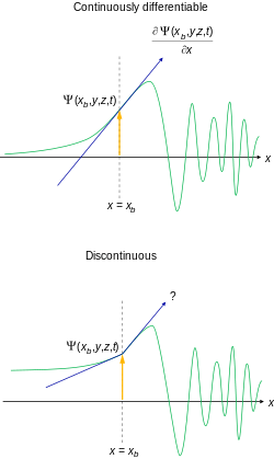
- It must be everywhere continuous and everywhere continuously differentiable. This is motivated by the appearance of the Schrödinger equation for most physically reasonable potentials.
It is possible to relax these conditions somewhat for special purposes.[nb 10] If these requirements are not met, it is not possible to interpret the wave function as a probability amplitude.[40]
This does not alter the structure of the Hilbert space that these particular wave functions inhabit, but it should be pointed out that the subspace of the square-integrable functions L2, which is a Hilbert space, satisfying the second requirement is not closed in L2, hence not a Hilbert space in itself.[nb 11] The functions that does not meet the requirements are still needed for both technical and practical reasons.[nb 12][nb 13]
More on wave functions and abstract state space
As has been demonstrated, the set of all possible wave functions in some representation for a system constitute an in general infinite-dimensional Hilbert space. Due to the multiple possible choices of representation basis, these Hilbert spaces are not unique. One therefore talks about an abstract Hilbert space, state space, where the choice of representation and basis is left undetermined. Specifically, each state is represented as an abstract vector in state space.[41] A quantum state |Ψ⟩ in any representation is generally expressed as a vector

where α = (α1, α2, ..., αn) are (dimensionless) discrete quantum numbers, and ω = (ω1, ω2, ..., ωm) are continuous variables (not necessarily dimensionless). All of them index the components of the vector, and |α, ω⟩ are the basis vectors in this representation. All α are in an n-dimensional set A = A1 × A2 × ... An where each Ai is the set of allowed values for αi, likewise all ω are in an m-dimensional "volume" Ω ⊆ ℝm where Ω = Ω1 × Ω2 × ... Ωm and each Ωi ⊆ ℝ is the set of allowed values for ωi, a subset of the real numbers ℝ. For generality n and m are not necessarily equal.
For example, for a single particle in 3d with spin s, neglecting other degrees of freedom, using Cartesian coordinates, we could take α = (sz) for the spin quantum number of the particle along the z direction, and ω = (x, y, z) for the particle's position coordinates. Here A = {−s, −s + 1, ..., s − 1, s} is the set of allowed spin quantum numbers and Ω = ℝ3 is the set of all possible particle positions throughout 3d position space. An alternative choice is α = (sy) for the spin quantum number along the y direction and ω = (px, py, pz) for the particle's momentum components. In this case A and Ω are the same.
Then, a component Ψ(α, ω, t) of the vector |Ψ⟩ is referred to as the "wave function" of the system.
When interpreted as a probability amplitude (non-relativistic systems with constant number of particles), the probability density of finding the system at α, ω is

The probability of finding system with α in some or all possible discrete-variable configurations, D ⊆ A, and ω in some or all possible continuous-variable configurations, C ⊆ Ω, is the sum and integral over the density,[nb 14]

where dmω = dω1dω2...dωm is a "differential volume element" in the continuous degrees of freedom. Since the sum of all probabilities must be 1, the normalization condition

must hold at all times during the evolution of the system.
The normalisation condition requires ρ dmω to be dimensionless, by dimensional analysis Ψ must have the same units as (ω1ω2...ωm)−1/2.
Ontology
Whether the wave function really exists, and what it represents, are major questions in the interpretation of quantum mechanics. Many famous physicists of a previous generation puzzled over this problem, such as Schrödinger, Einstein and Bohr. Some advocate formulations or variants of the Copenhagen interpretation (e.g. Bohr, Wigner and von Neumann) while others, such as Wheeler or Jaynes, take the more classical approach[42] and regard the wave function as representing information in the mind of the observer, i.e. a measure of our knowledge of reality. Some, including Schrödinger, Bohm and Everett and others, argued that the wave function must have an objective, physical existence. Einstein thought that a complete description of physical reality should refer directly to physical space and time, as distinct from the wave function, which refers to an abstract mathematical space.[43]
See also
- Boson
- de Broglie–Bohm theory
- Double-slit experiment
- Faraday wave
- Fermion
- Schrödinger equation
- Wave function collapse
- Wave packet
- Phase space formulation of quantum mechanics, wave functions are replaced by quasi-probability distributions that place the position and momenta variables on equal footing.
Remarks
- ↑ The functions are here assumed to be elements of L2, the space of square integrable functions. The elements of this space are more precisely equivalence classes of square integrable functions, two functions declared equivalent if they differ on a set of Lebesgue measure 0. This is necessary to obtain an inner product (that is, (Ψ, Ψ) = 0 ⇒ Ψ ≡ 0) as opposed to a semi-inner product. The integral is taken to be the Lebesque integral. This is essential for completeness of the space, thus yielding a complete inner product space = Hilbert space.
- ↑ The Fourier transform viewed as a unitary operator on the space L2 has eigenvalues ±1, ±i. The eigenvectors are "Hermite functions", i.e. Hermite polynomials multiplied by a Gaussian function. See Byron & Fuller (1992) for a description of the Fourier transform as a unitary transformation. For eigenvalues and eigenvalues, refer to Problem 27 Ch. 9.
- ↑ Column vectors can be motivated by the convenience of expressing the spin operator for a given spin as a matrix, for the z-component spin operator (divided by hbar to nondimensionalize)
- ↑ Each |sz⟩ is usually identified as a column vector
- ↑ For this statement to make sense, the observables need to be elements of a maximal commuting set. To see this, it is a simple matter to note that, for example, the momentum operator of the i'th particle in a n-particle system is not a generator of any symmetry in nature. On the other hand, the total momentum is a generator of a symmetry in nature; the translational symmetry.
- ↑ The resulting basis may or may not technically be a basis in the mathematical sense of Hilbert spaces. For instance, states of definite position and definite momentum are not square integrable. This may be overcome with the use of wave packets or by enclosing the system in a "box". See further remarks below.
- ↑ In technical terms, this is formulated the following way. The inner product yields a norm. This norm in turn induces a metric. If this metric is complete, then the aforementioned limits will be in the function space. The inner product space is then called complete. A complete inner product space is a Hilbert space. The abstract state space is always taken as a Hilbert space. The matching requirement for the function spaces is a natural one. The Hilbert space property of the abstract state space was originally extracted from the observation that the function spaces forming normalizable solutions to the Schrödinger equation are Hilbert spaces.
- ↑ As is explained in a later footnote, the integral must be taken to be the Lebesgue integral, the Riemann integral is not sufficient.
- ↑ Conway 1990. This means that inner products, hence norms, are preserved and that the mapping is a bounded, hence continuous, linear bijection. The property of completeness is preserved as well. Thus this is the right concept of isomorphism in the category of Hilbert spaces.
- ↑ One such relaxation is that the wave function must belong to the Sobolev space W1,2. It means that it is differentiable in the sense of distributions, and its gradient is square-integrable. This relaxation is necessary for potentials that are not functions but are distributions, such as the Dirac delta function.
- ↑ It is easy to visualize a sequence of functions meeting the requirement that converges to a discontinuous function. For this, modify an example given in Inner product space#Examples. This element though is an element of L2.
- ↑ For instance, in perturbation theory one may construct a sequence of functions approximating the true wave function. This sequence will be guaranteed to converge in a larger space, but without the assumption of a full-fledged Hilbert space, it will not be guaranteed that the convergence is to a function in the relevant space and hence solving the original problem.
- ↑ Some functions not being square-integrable, like the plane-wave free particle solutions are necessary for the description as outlined in a previous note and also further below.
- ↑ Here


Notes
- ↑ Born 1927, pp. 354–357
- ↑ Heisenberg 1958, p. 143
- ↑ Heisenberg, W. (1927/1985/2009). Heisenberg is translated by Camilleri 2009, p. 71, (from Bohr 1985, p. 142).
- ↑ Murdoch 1987, p. 43
- ↑ de Broglie 1960, p. 48
- ↑ Landau & Lifshitz, p. 6
- ↑ Newton 2002, pp. 19–21
- 1 2 3 4 Born 1926a, translated in Wheeler & Zurek 1983 at pages 52–55.
- 1 2 Born 1926b, translated in Ludwig 1968, pp. 206–225. Also here.
- ↑ Born, M. (1954).
- ↑ Einstein 1905, pp. 132–148 (in German), Arons & Peppard 1965, p. 367 (in English)
- ↑ Einstein 1916, pp. 47–62 and a nearly identical version Einstein 1917, pp. 121–128 translated in ter Haar 1967, pp. 167–183.
- ↑ de Broglie 1923, pp. 507–510,548,630
- ↑ Hanle 1977, pp. 606–609
- ↑ Schrödinger 1926, pp. 1049–1070
- ↑ Tipler, Mosca & Freeman 2008
- 1 2 3 Weinberg 2013
- ↑ Young & Freedman 2008, p. 1333
- 1 2 3 Atkins 1974
- ↑ Martin & Shaw 2008
- ↑ Pauli 1927, pp. 601–623.
- ↑ Weinberg (2002) takes the standpoint that quantum field theory appears the way it does because it is the only way to reconcile quantum mechanics with special relativity.
- ↑ Weinberg (2002) See especially chapter 5, where some of these results are derived.
- ↑ Weinberg 2002 Chapter 4.
- ↑ Zwiebach 2009
- ↑ Shankar 1994, Ch. 1
- 1 2 Griffiths 2004
- ↑ Shankar 1994, p. 378–379
- ↑ Landau & Lifshitz 1977
- ↑ Zettili 2009, p. 463
- ↑ Weinberg 2002 Chapter 3, Scattering matrix.
- ↑ Physics for Scientists and Engineers – with Modern Physics (6th Edition), P. A. Tipler, G. Mosca, Freeman, 2008, ISBN 0-7167-8964-7
- ↑ David Griffiths (2008). Introduction to elementary particles. Wiley-VCH. pp. 162–. ISBN 978-3-527-40601-2. Retrieved 27 June 2011.
- ↑ Weinberg 2002
- ↑ Weinberg 2002, Chapter 3
- ↑ Conway 1990
- ↑ Greiner & Reinhardt 2008
- ↑ Eisberg & Resnick 1985
- ↑ Rae 2008
- ↑ Atkins 1974, p. 258
- ↑ Dirac 1982
- ↑ Jaynes 2003
- ↑ Einstein 1998, p. 682
References
- Atkins, P. W. (1974). Quanta: A Handbook of Concepts. ISBN 0-19-855494-X.
- Arons, A. B.; Peppard, M. B. (1965). "Einstein's proposal of the photon concept: A translation of the Annalen der Physik paper of 1905" (PDF). American Journal of Physics. 33 (5): 367. Bibcode:1965AmJPh..33..367A. doi:10.1119/1.1971542.
- Bohr, N. (1985). J. Kalckar, ed. Niels Bohr - Collected Works: Foundations of Quantum Physics I (1926 - 1932). 6. Amsterdam: North Holland. ISBN 9780444532893.
- Born, M. (1926a). "Zur Quantenmechanik der Stoßvorgange". Z. Phys. 37: 863–867. Bibcode:1926ZPhy...37..863B. doi:10.1007/bf01397477.
- Born, M. (1926b). "Quantenmechanik der Stoßvorgange". Z. Phys. 38: 803–827. Bibcode:1926ZPhy...38..803B. doi:10.1007/bf01397184.
- Born, M. (1927). "Physical aspects of quantum mechanics". Nature. 119: 354–357. Bibcode:1927Natur.119..354B. doi:10.1038/119354a0.
- Born, M. (1954). "The statistical interpretation of quantum mechanics" (PDF). Nobel Lecture. December 11, 1954.
- de Broglie, L. (1923). "Radiations—Ondes et quanta" [Radiation—Waves and quanta]. Comptes Rendus (in French). 177: 507–510, 548, 630. Online copy (French) Online copy (English)
- de Broglie, L. (1960). Non-linear Wave Mechanics: a Causal Interpretation. Amsterdam: Elsevier.
- Camilleri, K. (2009). Heisenberg and the Interpretation of Quantum Mechanics: the Physicist as Philosopher. Cambridge UK: Cambridge University Press. ISBN 978-0-521-88484-6.
- Byron, F. W.; Fuller, R. W. (1992) [1969]. Mathematics of Classical and Quantum Physics. Dover Books on Physics (revised ed.). Dover Publications. ISBN 978-0-486-67164-2.
- Conway, J. B. (1990). A Course in Functional Analysis. Graduate Texts in Mathematics. 96. Springer Verlag. ISBN 0-387-97245-5.
- Dirac, P. A. M. (1982). The principles of quantum mechanics. The international series on monographs on physics (4th ed.). Oxford University Press. ISBN 0 19 852011 5.
- Dirac, P. A. M. (1939). "A new notation for quantum mechanics". Mathematical Proceedings of the Cambridge Philosophical Society. 35 (3): 416–418. Bibcode:1939PCPS...35..416D. doi:10.1017/S0305004100021162.
- Einstein, A. (1905). "Über einen die Erzeugung und Verwandlung des Lichtes betreffenden heuristischen Gesichtspunkt". Annalen der Physik (in German). 17 (6): 132–148. Bibcode:1905AnP...322..132E. doi:10.1002/andp.19053220607.
- Einstein, A. (1916). "Zur Quantentheorie der Strahlung". Mitteilungen der Physikalischen Gesellschaft Zürich. 18: 47–62.
- Einstein, A. (1917). "Zur Quantentheorie der Strahlung". Physikalische Zeitschrift (in German). 18: 121–128. Bibcode:1917PhyZ...18..121E.
- Einstein, A. (1998). P. A. Schlipp, ed. Albert Einstein: Philosopher-Scientist. The Library of Living Philosophers. VII (3rd ed.). La Salle Publishing Company, Illinois: Open Court. ISBN 0-87548-133-7.
- Eisberg, R.; Resnick, R. (1985). Quantum Physics of Atoms, Molecules, Solids, Nuclei and Particles (2nd ed.). John Wiley & Sons. ISBN 978-0-471-87373-0.
- Greiner, W.; Reinhardt, J. (2008). Quantum Electrodynamics (4th ed.). springer. ISBN 9783540875604.
- Griffiths, D. J. (2004). Introduction to Quantum Mechanics (2nd ed.). Essex England: Pearson Education Ltd. ISBN 978-0131118928.
- Heisenberg, W. (1958). Physics and Philosophy: the Revolution in Modern Science. New York: Harper & Row.
- Hanle, P.A. (1977), "Erwin Schrodinger's Reaction to Louis de Broglie's Thesis on the Quantum Theory.", Isis, 68 (4), doi:10.1086/351880
- Jaynes, E. T. (2003). G. Larry Bretthorst, ed. Probability Theory: The Logic of Science. Cambridge University Press. ISBN 978-0-521 59271-0.
- Landau, L.D.; Lifshitz, E. M. (1977). Quantum Mechanics: Non-Relativistic Theory. Vol. 3 (3rd ed.). Pergamon Press. ISBN 978-0-08-020940-1. Online copy
- Lerner, R.G.; Trigg, G.L. (1991). Encyclopaedia of Physics (2nd ed.). VHC Publishers. ISBN 0-89573-752-3.
- Ludwig, G. (1968). Wave Mechanics. Oxford UK: Pergamon Press. ISBN 0-08-203204-1. LCCN 66-30631.
- Murdoch, D. (1987). Niels Bohr's Philosophy of Physics. Cambridge UK: Cambridge University Press. ISBN 0-521-33320-2.
- Newton, R.G. (2002). Quantum Physics: a Text for Graduate Student. New York: Springer. ISBN 0-387-95473-2.
- Pauli, Wolfgang (1927). "Zur Quantenmechanik des magnetischen Elektrons". Zeitschrift für Physik (in German). 43. Bibcode:1927ZPhy...43..601P. doi:10.1007/bf01397326.
- Peleg, Y.; Pnini, R.; Zaarur, E.; Hecht, E. (2010). Quantum mechanics. Schaum's outlines (2nd ed.). McGraw Hill. ISBN 978-0-07-162358-2.
- Rae, A.I.M. (2008). Quantum Mechanics. 2 (5th ed.). Taylor & Francis Group. ISBN 1-5848-89705.
- Schrödinger, E. (1926). "An Undulatory Theory of the Mechanics of Atoms and Molecules" (PDF). Physical Review. 28 (6): 1049–1070. Bibcode:1926PhRv...28.1049S. doi:10.1103/PhysRev.28.1049. Archived from the original (PDF) on 17 December 2008.
- Shankar, R. (1994). Principles of Quantum Mechanics (2nd ed.). ISBN 0306447908.
- Martin, B.R.; Shaw, G. (2008). Particle Physics. Manchester Physics Series (3rd ed.). John Wiley & Sons. ISBN 978-0-470-03294-7.
- ter Haar, D. (1967). The Old Quantum Theory. Pergamon Press. pp. 167–183. LCCN 66029628.
- Tipler, P. A.; Mosca, G.; Freeman (2008). Physics for Scientists and Engineers – with Modern Physics (6th ed.). ISBN 0-7167-8964-7.
- Weinberg, S. (2013), Lectures in Quantum Mechanics, Cambridge University Press, ISBN 978-1-107-02872-2
- Weinberg, S. (2002), The Quantum Theory of Fields, 1, Cambridge University Press, ISBN 0-521-55001-7
- Young, H. D.; Freedman, R. A. (2008). Pearson, ed. Sears' and Zemansky's University Physics (12th ed.). Addison-Wesley. ISBN 978-0-321-50130-1.
- Wheeler, J.A.; Zurek, W.H. (1983). Quantum Theory and Measurement. Princeton NJ: Princeton University Press.
- Zettili, N. (2009). Quantum Mechanics: Concepts and Applications (2nd ed.). ISBN 978-0-470-02679-3.
- Zwiebach, Barton (2009). A First Course in String Theory. Cambridge University Press. ISBN 978-0-521-88032-9.
Further reading
- Yong-Ki Kim (September 2, 2000). "Practical Atomic Physics" (PDF). National Institute of Standards and Technology. Maryland: 1 (55 pages). Archived from the original (PDF) on July 22, 2011. Retrieved 2010-08-17.
- Polkinghorne, John (2002). Quantum Theory, A Very Short Introduction. Oxford University Press. ISBN 0-19-280252-6.
External links
- , , ,
- Normalization.
- Quantum Mechanics and Quantum Computation at BerkeleyX
- Einstein, The quantum theory of radiation