Polynomial
In mathematics, a polynomial is an expression consisting of variables (or indeterminates) and coefficients, that involves only the operations of addition, subtraction, multiplication, and non-negative integer exponents. An example of a polynomial of a single indeterminate x is x2 − 4x + 7. An example in three variables is x3 + 2xyz2 − yz + 1.
Polynomials appear in a wide variety of areas of mathematics and science. For example, they are used to form polynomial equations, which encode a wide range of problems, from elementary word problems to complicated problems in the sciences; they are used to define polynomial functions, which appear in settings ranging from basic chemistry and physics to economics and social science; they are used in calculus and numerical analysis to approximate other functions. In advanced mathematics, polynomials are used to construct polynomial rings and algebraic varieties, central concepts in algebra and algebraic geometry.
Etymology
The word polynomial joins two diverse roots: the Greek poly, meaning "many," and the Latin nomen, or name. It was derived from the term binomial by replacing the Latin root bi- with the Greek poly-. The word polynomial was first used in the 17th century.[1]
Notation and terminology
The x occurring in a polynomial is commonly called either a variable or an indeterminate. When the polynomial is considered as an expression, x is a fixed symbol which does not have any value (its value is "indeterminate"). It is thus more correct to call it an "indeterminate". However, when one considers the function defined by the polynomial, then x represents the argument of the function, and is therefore called a "variable". Many authors use these two words interchangeably.
It is a common convention to use uppercase letters for the indeterminates and the corresponding lowercase letters for the variables (arguments) of the associated function.
It may be confusing that a polynomial P in the indeterminate x may appear in the formulas either as P or as P(x).
Normally, the name of the polynomial is P, not P(x). However, if a denotes a number, a variable, another polynomial, or, more generally any expression, then P(a) denotes, by convention, the result of substituting x by a in P. Thus, the polynomial P defines the function

which is the polynomial function associated to P.
Frequently, when using this function, one supposes that a is a number. However one may use it over any domain where addition and multiplication are defined (any ring). In particular, when a is the indeterminate x, then the image of x by this function is the polynomial P itself (substituting x to x does not change anything). In other words,

This equality allows writing "let P(x) be a polynomial" as a shorthand for "let P be a polynomial in the indeterminate x". On the other hand, when it is not necessary to emphasize the name of the indeterminate, many formulas are much simpler and easier to read if the name(s) of the indeterminate(s) do not appear at each occurrence of the polynomial.
Definition
A polynomial is an expression that can be built from constants and symbols called indeterminates or variables by means of addition, multiplication and exponentiation to a non-negative power. Two such expressions that may be transformed, one to the other, by applying the usual properties of commutativity, associativity and distributivity of addition and multiplication are considered as defining the same polynomial.
A polynomial in a single indeterminate x can always be written (or rewritten) in the form

where are constants and is the indeterminate. The word "indeterminate" means that represents no particular value, although any value may be substituted for it. The mapping that associates the result of this substitution to the substituted value is a function, called a polynomial function.


This can be expressed more concisely by using summation notation:

That is, a polynomial can either be zero or can be written as the sum of a finite number of non-zero terms. Each term consists of the product of a number—called the coefficient of the term[2]—and a finite number of indeterminates, raised to nonnegative integer powers. The exponent on an indeterminate in a term is called the degree of that indeterminate in that term; the degree of the term is the sum of the degrees of the indeterminates in that term, and the degree of a polynomial is the largest degree of any one term with nonzero coefficient. Because x = x1, the degree of an indeterminate without a written exponent is one.
A term and a polynomial with no indeterminates are called, respectively, a constant term and a constant polynomial.[3] The degree of a constant term and of a nonzero constant polynomial is 0. The degree of the zero polynomial, 0, (which has no terms at all) is generally treated as not defined (but see below).[4]
For example:

is a term. The coefficient is −5, the indeterminates are x and y, the degree of x is two, while the degree of y is one. The degree of the entire term is the sum of the degrees of each indeterminate in it, so in this example the degree is 2 + 1 = 3.
Forming a sum of several terms produces a polynomial. For example, the following is a polynomial:

It consists of three terms: the first is degree two, the second is degree one, and the third is degree zero.
Polynomials of small degree have been given specific names. A polynomial of degree zero is a constant polynomial or simply a constant. Polynomials of degree one, two or three are respectively linear polynomials, quadratic polynomials and cubic polynomials. For higher degrees the specific names are not commonly used, although quartic polynomial (for degree four) and quintic polynomial (for degree five) are sometimes used. The names for the degrees may be applied to the polynomial or to its terms. For example, in x2 + 2x + 1 the term 2x is a linear term in a quadratic polynomial.
The polynomial 0, which may be considered to have no terms at all, is called the zero polynomial. Unlike other constant polynomials, its degree is not zero. Rather the degree of the zero polynomial is either left explicitly undefined, or defined as negative (either −1 or −∞).[5] These conventions are useful when defining Euclidean division of polynomials. The zero polynomial is also unique in that it is the only polynomial having an infinite number of roots. The graph of the zero polynomial, f(x) = 0, is the X-axis.
In the case of polynomials in more than one indeterminate, a polynomial is called homogeneous of degree n if all its non-zero terms have degree n. The zero polynomial is homogeneous, and, as homogeneous polynomial, its degree is undefined.[6] For example, x3y2 + 7x2y3 − 3x5 is homogeneous of degree 5. For more details, see homogeneous polynomial.
The commutative law of addition can be used to rearrange terms into any preferred order. In polynomials with one indeterminate, the terms are usually ordered according to degree, either in "descending powers of x", with the term of largest degree first, or in "ascending powers of x". The polynomial in the example above is written in descending powers of x. The first term has coefficient 3, indeterminate x, and exponent 2. In the second term, the coefficient is −5. The third term is a constant. Because the degree of a non-zero polynomial is the largest degree of any one term, this polynomial has degree two.[7]
Two terms with the same indeterminates raised to the same powers are called "similar terms" or "like terms", and they can be combined, using the distributive law, into a single term whose coefficient is the sum of the coefficients of the terms that were combined. It may happen that this makes the coefficient 0.[8] Polynomials can be classified by the number of terms with nonzero coefficients, so that a one-term polynomial is called a monomial,[9] a two-term polynomial is called a binomial, and a three-term polynomial is called a trinomial. The term "quadrinomial" is occasionally used for a four-term polynomial.
A polynomial in one indeterminate is called a univariate polynomial, a polynomial in more than one indeterminate is called a multivariate polynomial. A polynomial with two indeterminates is called a bivariate polynomial. These notions refer more to the kind of polynomials one is generally working with than to individual polynomials; for instance when working with univariate polynomials one does not exclude constant polynomials (which may result, for instance, from the subtraction of non-constant polynomials), although strictly speaking constant polynomials do not contain any indeterminates at all. It is possible to further classify multivariate polynomials as bivariate, trivariate, and so on, according to the maximum number of indeterminates allowed. Again, so that the set of objects under consideration be closed under subtraction, a study of trivariate polynomials usually allows bivariate polynomials, and so on. It is common, also, to say simply "polynomials in x, y, and z", listing the indeterminates allowed.
The evaluation of a polynomial consists of substituting a numerical value to each indeterminate and carrying out the indicated multiplications and additions. For polynomials in one indeterminate, the evaluation is usually more efficient (lower number of arithmetic operations to perform) using Horner's method:

Arithmetic
Polynomials can be added using the associative law of addition (grouping all their terms together into a single sum), possibly followed by reordering, and combining of like terms.[8][10] For example, if

then

which can be simplified to

To work out the product of two polynomials into a sum of terms, the distributive law is repeatedly applied, which results in each term of one polynomial being multiplied by every term of the other.[8] For example, if

then

which can be simplified to

Polynomial evaluation can be used to compute the remainder of polynomial division by a polynomial of degree one, because the remainder of the division of f(x) by (x − a) is f(a); see the polynomial remainder theorem. This is more efficient than the usual algorithm of division when the quotient is not needed.
- A sum of polynomials is a polynomial.[4]
- A product of polynomials is a polynomial.[4]
- A composition of two polynomials is a polynomial, which is obtained by substituting a variable of the first polynomial by the second polynomial.[4]
- The derivative of the polynomial anxn + an−1xn−1 + ... + a2x2 + a1x + a0 is the polynomial nanxn−1 + (n−1)an−1xn−2 + ... + 2a2x + a1. If the set of the coefficients does not contain the integers (for example if the coefficients are integers modulo some prime number p), then kak should be interpreted as the sum of ak with itself, k times. For example, over the integers modulo p, the derivative of the polynomial xp + 1 is the polynomial 0.[11]
- A primitive integral or antiderivative of the polynomial anxn + an−1xn−1 + ... + a2x2 + a1x + a0 is the polynomial anxn+1/(n+1) + an−1xn/n + ... + a2x3/3 + a1x2/2 + a0x + c, where c is an arbitrary constant. For instance, the antiderivatives of x2 + 1 have the form 1/3x3 + x + c.
As for the integers, two kinds of divisions are considered for the polynomials. The Euclidean division of polynomials that generalizes the Euclidean division of the integers. It results in two polynomials, a quotient and a remainder that are characterized by the following property of the polynomials: given two polynomials a and b such that b ≠ 0, there exists a unique pair of polynomials, q, the quotient, and r, the remainder, such that a = b q + r and degree(r) < degree(b) (here the polynomial zero is supposed to have a negative degree). By hand as well as with a computer, this division can be computed by the polynomial long division algorithm.[12]
All polynomials with coefficients in a unique factorization domain (for example, the integers or a field) also have a factored form in which the polynomial is written as a product of irreducible polynomials and a constant. This factored form is unique up to the order of the factors and their multiplication by an invertible constant. In the case of the field of complex numbers, the irreducible factors are linear. Over the real numbers, they have the degree either one or two. Over the integers and the rational numbers the irreducible factors may have any degree.[13] For example, the factored form of

is

over the integers and the reals and

over the complex numbers.
The computation of the factored form, called factorization is, in general, too difficult to be done by hand-written computation. However, efficient polynomial factorization algorithms are available in most computer algebra systems.
A formal quotient of polynomials, that is, an algebraic fraction wherein the numerator and denominator are polynomials, is called a "rational expression" or "rational fraction" and is not, in general, a polynomial. Division of a polynomial by a number, however, yields another polynomial. For example, x3/12 is considered a valid term in a polynomial (and a polynomial by itself) because it is equivalent to (1/12)x3 and 1/12 is just a constant. When this expression is used as a term, its coefficient is therefore 1/12. For similar reasons, if complex coefficients are allowed, one may have a single term like (2 + 3i) x3; even though it looks like it should be expanded to two terms, the complex number 2 + 3i is one complex number, and is the coefficient of that term. The expression 1/(x2 + 1) is not a polynomial because it includes division by a non-constant polynomial. The expression (5 + y)x is not a polynomial, because it contains an indeterminate used as exponent.
Because subtraction can be replaced by addition of the opposite quantity, and because positive integer exponents can be replaced by repeated multiplication, all polynomials can be constructed from constants and indeterminates using only addition and multiplication.
Polynomial functions
A polynomial function is a function that can be defined by evaluating a polynomial. A function f of one argument is thus a polynomial function if it satisfies.

for all arguments x, where n is a non-negative integer and a0, a1, a2, ..., an are constant coefficients.
For example, the function f, taking real numbers to real numbers, defined by

is a polynomial function of one variable. Polynomial functions of multiple variables are similarly defined, using polynomials in multiple indeterminates, as in

An example is also the function which, although it does not look like a polynomial, is a polynomial function on because for every from it is true that (see Chebyshev polynomials).

![[-1,1]](../I/m/51e3b7f14a6f70e614728c583409a0b9a8b9de01.svg)

Polynomial functions are a class of functions having many important properties. They are all continuous, smooth, entire, computable, etc.
Graphs
 Polynomial of degree 2:
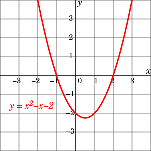
f(x) = x2 − x − 2
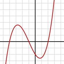
= (x + 1)(x − 2)- Polynomial of degree 3:
f(x) = x3/4 + 3x2/4 − 3x/2 − 2
= 1/4 (x + 4)(x + 1)(x − 2) 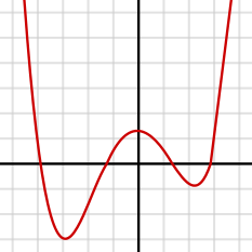 Polynomial of degree 4:
f(x) = 1/14 (x + 4)(x + 1)(x − 1)(x − 3)
+ 0.5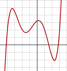 Polynomial of degree 5:
f(x) = 1/20 (x + 4)(x + 2)(x + 1 )(x − 1)
(x − 3)+ 2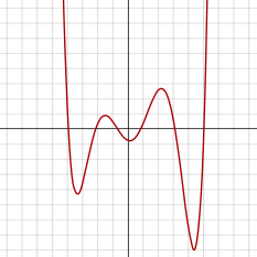 Polynomial of degree 6:
f(x) = 1/100 (x6 − 2x 5 − 26x4 + 28x3
+ 145x2 - 26x - 80)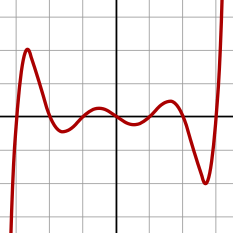 Polynomial of degree 7:
f(x) = (x − 3)(x − 2)(x − 1)(x)(x + 1)(x + 2)
(x + 3)
A polynomial function in one real variable can be represented by a graph.
- The graph of the zero polynomial
- f(x) = 0
- is the x-axis.
- The graph of a degree 0 polynomial
- f(x) = a0, where a0 ≠ 0,
- is a horizontal line with y-intercept a0
- The graph of a degree 1 polynomial (or linear function)
- f(x) = a0 + a1x , where a1 ≠ 0,
- is an oblique line with y-intercept a0 and slope a1.
- The graph of a degree 2 polynomial
- f(x) = a0 + a1x + a2x2, where a2 ≠ 0
- is a parabola.
- The graph of a degree 3 polynomial
- f(x) = a0 + a1x + a2x2 + a3x3, where a3 ≠ 0
- is a cubic curve.
- The graph of any polynomial with degree 2 or greater
- f(x) = a0 + a1x + a2x2 + ... + anxn , where an ≠ 0 and n ≥ 2
- is a continuous non-linear curve.
A non constant polynomial function tends to infinity when the variable increases indefinitely (in absolute value). If the degree is higher than one, the graph does not have any asymptote. It has two parabolic branches with vertical direction (one branch for positive x and one for negative x).
Polynomial graphs are analyzed in calculus using intercepts, slopes, concavity, and end behavior.
Equations
A polynomial equation, also called algebraic equation, is an equation of the form[14]

For example,

is a polynomial equation.
In case of a univariate polynomial equation, the variable is considered an unknown, and one seeks to find the possible values for which both members of the equation evaluate to the same value (in general more than one solution may exist). A polynomial equation stands in contrast to a polynomial identity like (x + y)(x − y) = x2 − y2, where both expressions represent the same polynomial in different forms, and as a consequence any evaluation of both members gives a valid equality.
In elementary algebra, methods such as the quadratic formula are given for solving all first degree and second degree polynomial equations in one variable. There are also formulas for the cubic and quartic equations. For higher degrees, the Abel–Ruffini theorem asserts that there can not exist a general formula in radicals. However, root-finding algorithms may be used to find numerical approximations of the roots of a polynomial expression of any degree.
The number of real solutions of a polynomial equation with real coefficients may not exceed the degree, and equals the degree when the complex solutions are counted with their multiplicity. This fact is called the fundamental theorem of algebra.
Solving equations
Every polynomial P in x corresponds to a function, f(x) = P (where the occurrences of x in P are interpreted as the argument of f), called the polynomial function of P; the equation in x setting f(x) = 0 is the polynomial equation corresponding to P. The solutions of this equation are called the roots of the polynomial; they are the zeroes of the function f (corresponding to the points where the graph of f meets the x-axis). A number a is a root of P if and only if the polynomial x − a (of degree one in x) divides P. It may happen that x − a divides P more than once: if (x − a)2 divides P then a is called a multiple root of P, and otherwise a is called a simple root of P. If P is a nonzero polynomial, there is a highest power m such that (x − a)m divides P, which is called the multiplicity of the root a in P. When P is the zero polynomial, the corresponding polynomial equation is trivial, and this case is usually excluded when considering roots: with the above definitions every number would be a root of the zero polynomial, with undefined (or infinite) multiplicity. With this exception made, the number of roots of P, even counted with their respective multiplicities, cannot exceed the degree of P.[15] The relation between the roots of a polynomial and its coefficients is described by Vieta's formulas.
Some polynomials, such as x2 + 1, do not have any roots among the real numbers. If, however, the set of allowed candidates is expanded to the complex numbers, every non-constant polynomial has at least one root; this is the fundamental theorem of algebra. By successively dividing out factors x − a, one sees that any polynomial with complex coefficients can be written as a constant (its leading coefficient) times a product of such polynomial factors of degree 1; as a consequence, the number of (complex) roots counted with their multiplicities is exactly equal to the degree of the polynomial.
There is a difference between approximating roots and finding exact expressions for roots. Formulas for expressing the roots of polynomials of degree 2 in terms of square roots have been known since ancient times (see quadratic equation), and for polynomials of degree 3 or 4 similar formulas (using cube roots in addition to square roots) were found in the 16th century (see cubic function and quartic function for the formulas and Niccolò Fontana Tartaglia, Lodovico Ferrari, Gerolamo Cardano, and François Viète for historical details). But formulas for degree 5 eluded researchers for several centuries. In 1824, Niels Henrik Abel proved the striking result that there can be no general (finite) formula, involving only arithmetic operations and radicals, that expresses the roots of a polynomial of degree 5 or greater in terms of its coefficients (see Abel–Ruffini theorem). In 1830, Évariste Galois, studying the permutations of the roots of a polynomial, extended the Abel–Ruffini theorem by showing that, given a polynomial equation, one may decide whether it is solvable by radicals, and, if it is, solve it. This result marked the start of Galois theory and group theory, two important branches of modern mathematics. Galois himself noted that the computations implied by his method were impracticable. Nevertheless, formulas for solvable equations of degrees 5 and 6 have been published (see quintic function and sextic equation).
Numerical approximation of roots of polynomials in one unknown is easily done on a computer by the Jenkins–Traub method, Laguerre's method, Durand–Kerner method, or by some other root-finding algorithm.[16]
For polynomials in more than one indeterminate the notion of root does not exist, and there are usually infinitely many combinations of values for the variables for which the polynomial function takes the value zero. However, for certain sets of such polynomials it may happen that for only finitely many combinations all polynomial functions take the value zero.
For a set of polynomial equations in several unknowns, there are algorithms to decide whether they have a finite number of complex solutions. If the number of solutions is finite, there are algorithms to compute the solutions. The methods underlying these algorithms are described in the article System of polynomial equations.
The special case where all the polynomials are of degree one is called a system of linear equations, for which another range of different solution methods exist, including the classical Gaussian elimination.
A polynomial equation for which one is interested only in the solutions which are integers is called a Diophantine equation. Solving Diophantine equations is a very hard task. It has been proved that there cannot be any general algorithm for solving them, and even for deciding whether the set of solutions is empty (see Hilbert's tenth problem). Some of the most famous problems that have been solved during the fifty last years are related to Diophantine equations, such as Fermat's Last Theorem.
Generalizations
There are several generalizations of the concept of polynomials.
Trigonometric polynomials
A trigonometric polynomial is a finite linear combination of functions sin(nx) and cos(nx) with n taking on the values of one or more natural numbers.[17] The coefficients may be taken as real numbers, for real-valued functions.
If sin(nx) and cos(nx) are expanded in terms of sin(x) and cos(x), a trigonometric polynomial becomes a polynomial in the two variables sin(x) and cos(x) (using List of trigonometric identities#Multiple-angle formulae). Conversely, every polynomial in sin(x) and cos(x) may be converted, with Product-to-sum identities, into a linear combination of functions sin(nx) and cos(nx). This equivalence explains why linear combinations are called polynomials.
For complex coefficients, there is no difference between such a function and a finite Fourier series.
Trigonometric polynomials are widely used, for example in trigonometric interpolation applied to the interpolation of periodic functions. They are used also in the discrete Fourier transform.
Matrix polynomials
A matrix polynomial is a polynomial with matrices as variables.[18] Given an ordinary, scalar-valued polynomial

this polynomial evaluated at a matrix A is

where I is the identity matrix.[19]
A matrix polynomial equation is an equality between two matrix polynomials, which holds for the specific matrices in question. A matrix polynomial identity is a matrix polynomial equation which holds for all matrices A in a specified matrix ring Mn(R).
Laurent polynomials
Laurent polynomials are like polynomials, but allow negative powers of the variable(s) to occur.
Rational functions
A rational fraction is the quotient (algebraic fraction) of two polynomials. Any algebraic expression that can be rewritten as a rational fraction is a rational function.
While polynomial functions are defined for all values of the variables, a rational function is defined only for the values of the variables for which the denominator is not zero.
The rational fractions include the Laurent polynomials, but do not limit denominators to powers of an indeterminate.
Power series
Formal power series are like polynomials, but allow infinitely many non-zero terms to occur, so that they do not have finite degree. Unlike polynomials they cannot in general be explicitly and fully written down (just like irrational numbers cannot), but the rules for manipulating their terms are the same as for polynomials. Non-formal power series also generalize polynomials, but the multiplication of two power series may not converge.
Other examples
- A bivariate polynomial where the second variable is substituted by an exponential function applied to the first variable, for example P(x, ex), may be called an exponential polynomial.
Applications
Calculus
The simple structure of polynomial functions makes them quite useful in analyzing general functions using polynomial approximations. An important example in calculus is Taylor's theorem, which roughly states that every differentiable function locally looks like a polynomial function, and the Stone–Weierstrass theorem, which states that every continuous function defined on a compact interval of the real axis can be approximated on the whole interval as closely as desired by a polynomial function.
Calculating derivatives and integrals of polynomial functions is particularly simple. For the polynomial function
the derivative with respect to x is

and the indefinite integral is

Abstract algebra
In abstract algebra, one distinguishes between polynomials and polynomial functions. A polynomial f in one indeterminate x over a ring R is defined as a formal expression of the form

where n is a natural number, the coefficients a0, . . ., an are elements of R, and x is a formal symbol, whose powers xi are just placeholders for the corresponding coefficients ai, so that the given formal expression is just a way to encode the sequence (a0, a1, . . .), where there is an n such that ai = 0 for all i > n. Two polynomials sharing the same value of n are considered equal if and only if the sequences of their coefficients are equal; furthermore any polynomial is equal to any polynomial with greater value of n obtained from it by adding terms in front whose coefficient is zero. These polynomials can be added by simply adding corresponding coefficients (the rule for extending by terms with zero coefficients can be used to make sure such coefficients exist). Thus each polynomial is actually equal to the sum of the terms used in its formal expression, if such a term aixi is interpreted as a polynomial that has zero coefficients at all powers of x other than xi. Then to define multiplication, it suffices by the distributive law to describe the product of any two such terms, which is given by the rule
- for all elements a, b of the ring R and all natural numbers k and l.

Thus the set of all polynomials with coefficients in the ring R forms itself a ring, the ring of polynomials over R, which is denoted by R[x]. The map from R to R[x] sending r to rx0 is an injective homomorphism of rings, by which R is viewed as a subring of R[x]. If R is commutative, then R[x] is an algebra over R.
One can think of the ring R[x] as arising from R by adding one new element x to R, and extending in a minimal way to a ring in which x satisfies no other relations than the obligatory ones, plus commutation with all elements of R (that is xr = rx). To do this, one must add all powers of x and their linear combinations as well.
Formation of the polynomial ring, together with forming factor rings by factoring out ideals, are important tools for constructing new rings out of known ones. For instance, the ring (in fact field) of complex numbers, which can be constructed from the polynomial ring R[x] over the real numbers by factoring out the ideal of multiples of the polynomial x2 + 1. Another example is the construction of finite fields, which proceeds similarly, starting out with the field of integers modulo some prime number as the coefficient ring R (see modular arithmetic).
If R is commutative, then one can associate to every polynomial P in R[x], a polynomial function f with domain and range equal to R (more generally one can take domain and range to be the same unital associative algebra over R). One obtains the value f(r) by substitution of the value R for the symbol x in P. One reason to distinguish between polynomials and polynomial functions is that over some rings different polynomials may give rise to the same polynomial function (see Fermat's little theorem for an example where R is the integers modulo p). This is not the case when R is the real or complex numbers, whence the two concepts are not always distinguished in analysis. An even more important reason to distinguish between polynomials and polynomial functions is that many operations on polynomials (like Euclidean division) require looking at what a polynomial is composed of as an expression rather than evaluating it at some constant value for x.
Divisibility
In commutative algebra, one major focus of study is divisibility among polynomials. If R is an integral domain and f and g are polynomials in R[x], it is said that f divides g or f is a divisor of g if there exists a polynomial q in R[x] such that f q = g. One can show that every zero gives rise to a linear divisor, or more formally, if f is a polynomial in R[x] and r is an element of R such that f(r) = 0, then the polynomial (x − r) divides f. The converse is also true. The quotient can be computed using the polynomial long division.[20][21]
If F is a field and f and g are polynomials in F[x] with g ≠ 0, then there exist unique polynomials q and r in F[x] with

and such that the degree of r is smaller than the degree of g (using the convention that the polynomial 0 has a negative degree). The polynomials q and r are uniquely determined by f and g. This is called Euclidean division, division with remainder or polynomial long division and shows that the ring F[x] is a Euclidean domain.
Analogously, prime polynomials (more correctly, irreducible polynomials) can be defined as non-zero polynomials which cannot be factorized into the product of two non constant polynomials. In the case of coefficients in a ring, "non constant" must be replaced by "non constant or non unit" (both definitions agree in the case of coefficients in a field). Any polynomial may be decomposed into the product of an invertible constant by a product of irreducible polynomials. If the coefficients belong to a field or a unique factorization domain this decomposition is unique up to the order of the factors and the multiplication of any non unit factor by a unit (and division of the unit factor by the same unit). When the coefficients belong to integers, rational numbers or a finite field, there are algorithms to test irreducibility and to compute the factorization into irreducible polynomials (see Factorization of polynomials). These algorithms are not practicable for hand written computation, but are available in any computer algebra system. Eisenstein's criterion can also be used in some cases to determine irreducibility.
Other applications
Polynomials serve to approximate other functions,[22] such as the use of splines.
Polynomials are frequently used to encode information about some other object. The characteristic polynomial of a matrix or linear operator contains information about the operator's eigenvalues. The minimal polynomial of an algebraic element records the simplest algebraic relation satisfied by that element. The chromatic polynomial of a graph counts the number of proper colourings of that graph.
The term "polynomial", as an adjective, can also be used for quantities or functions that can be written in polynomial form. For example, in computational complexity theory the phrase polynomial time means that the time it takes to complete an algorithm is bounded by a polynomial function of some variable, such as the size of the input.
History
Determining the roots of polynomials, or "solving algebraic equations", is among the oldest problems in mathematics. However, the elegant and practical notation we use today only developed beginning in the 15th century. Before that, equations were written out in words. For example, an algebra problem from the Chinese Arithmetic in Nine Sections, circa 200 BCE, begins "Three sheafs of good crop, two sheafs of mediocre crop, and one sheaf of bad crop are sold for 29 dou." We would write 3x + 2y + z = 29.
History of the notation
The earliest known use of the equal sign is in Robert Recorde's The Whetstone of Witte, 1557. The signs + for addition, − for subtraction, and the use of a letter for an unknown appear in Michael Stifel's Arithemetica integra, 1544. René Descartes, in La géometrie, 1637, introduced the concept of the graph of a polynomial equation. He popularized the use of letters from the beginning of the alphabet to denote constants and letters from the end of the alphabet to denote variables, as can be seen above, in the general formula for a polynomial in one variable, where the a's denote constants and x denotes a variable. Descartes introduced the use of superscripts to denote exponents as well.[23]
See also
- Lill's method
- List of polynomial topics
- Polynomials on vector spaces
- Power series
- Table of mathematical expressions
- Polynomial transformations
- Polynomiography
Notes
- ↑ See "polynomial" and "binomial", Compact Oxford English Dictionary
- ↑ The coefficient of a term may be any number from a specified set. If that set is the set of real numbers, we speak of "polynomials over the reals". Other common kinds of polynomials are polynomials with integer coefficients, polynomials with complex coefficients, and polynomials with coefficients that are integers modulo of some prime number p.
- ↑ This terminology dates from the time when the distinction was not clear between a polynomial and the function that it defines: a constant term and a constant polynomial define constant functions.
- 1 2 3 4 Barbeau, E.J. (2003). Polynomials. Springer. pp. 1–2. ISBN 978-0-387-40627-5.
- ↑ Weisstein, Eric W. "Zero Polynomial". MathWorld.
- ↑ In fact, as homogeneous function, it is homogeneous of every degree
- ↑ Edwards, Harold M. (1995). Linear Algebra. Springer. p. 78. ISBN 978-0-8176-3731-6.
- 1 2 3 Edwards, Harold M. (1995). Linear Algebra. Springer. p. 47. ISBN 978-0-8176-3731-6.
- ↑ Some authors use "monomial" to mean "monic monomial". See Knapp, Anthony W. (2007). Advanced Algebra: Along with a Companion Volume Basic Algebra. Springer. p. 457. ISBN 0-8176-4522-5.
- ↑ Salomon, David (2006). Coding for Data and Computer Communications. Springer. p. 459. ISBN 978-0-387-23804-3.
- ↑ Barbeau, E.J. (2003). Polynomials. Springer. pp. 64–5. ISBN 978-0-387-40627-5.
- ↑ Peter H. Selby, Steve Slavin, Practical Algebra: A Self-Teaching Guide, 2nd Edition, Wiley, ISBN 0-471-53012-3 ISBN 978-0-471-53012-1
- ↑ Barbeau, E.J. (2003). Polynomials. Springer. pp. 80–2. ISBN 978-0-387-40627-5.
- ↑ Proskuryakov, I.V. (1994). "Algebraic equation". In Hazewinkel, Michiel. Encyclopaedia of Mathematics. vol. 1. Springer. ISBN 978-1-55608-010-4.
- ↑ Leung,, Kam-tim; et al. (1992). Polynomials and Equations. Hong Kong University Press. p. 134. ISBN 9789622092716.
- ↑ McNamee, J.M. (2007). Numerical Methods for Roots of Polynomials, Part 1. Elsevier. ISBN 978-0-08-048947-6.
- ↑ Powell, Michael J. D. (1981). Approximation Theory and Methods. Cambridge University Press. ISBN 978-0-521-29514-7.
- ↑ Gohberg, Israel; Lancaster, Peter; Rodman, Leiba (2009) [1982]. Matrix Polynomials. Classics in Applied Mathematics. 58. Lancaster, PA: Society for Industrial and Applied Mathematics. ISBN 0-89871-681-0. Zbl 1170.15300.
- ↑ Horn & Johnson 1990, p. 36.
- ↑ Irving, Ronald S. (2004). Integers, Polynomials, and Rings: A Course in Algebra. Springer. p. 129. ISBN 978-0-387-20172-6.
- ↑ Jackson, Terrence H. (1995). From Polynomials to Sums of Squares. CRC Press. p. 143. ISBN 978-0-7503-0329-3.
- ↑ de Villiers, Johann (2012). Mathematics of Approximation. Springer. ISBN 9789491216503.
- ↑ Howard Eves, An Introduction to the History of Mathematics, Sixth Edition, Saunders, ISBN 0-03-029558-0
References
- Barbeau, E.J. (2003). Polynomials. Springer. ISBN 978-0-387-40627-5.
- Bronstein, Manuel; et al., eds. (2006). Solving Polynomial Equations: Foundations, Algorithms, and Applications. Springer. ISBN 978-3-540-27357-8.
- Cahen, Paul-Jean; Chabert, Jean-Luc (1997). Integer-Valued Polynomials. American Mathematical Society. ISBN 978-0-8218-0388-2.
- Lang, Serge (2002), Algebra, Graduate Texts in Mathematics, 211 (Revised third ed.), New York: Springer-Verlag, ISBN 978-0-387-95385-4, MR 1878556. This classical book covers most of the content of this article.
- Leung, Kam-tim; et al. (1992). Polynomials and Equations. Hong Kong University Press. ISBN 9789622092716.
- Mayr, K. Über die Auflösung algebraischer Gleichungssysteme durch hypergeometrische Funktionen. Monatshefte für Mathematik und Physik vol. 45, (1937) pp. 280–313.
- Prasolov, Victor V. (2005). Polynomials. Springer. ISBN 978-3-642-04012-2.
- Sethuraman, B.A. (1997). "Polynomials". Rings, Fields, and Vector Spaces: An Introduction to Abstract Algebra Via Geometric Constructibility. Springer. ISBN 978-0-387-94848-5.
- Umemura, H. Solution of algebraic equations in terms of theta constants. In D. Mumford, Tata Lectures on Theta II, Progress in Mathematics 43, Birkhäuser, Boston, 1984.
- von Lindemann, F. Über die Auflösung der algebraischen Gleichungen durch transcendente Functionen. Nachrichten von der Königl. Gesellschaft der Wissenschaften, vol. 7, 1884. Polynomial solutions in terms of theta functions.
- von Lindemann, F. Über die Auflösung der algebraischen Gleichungen durch transcendente Functionen II. Nachrichten von der Königl. Gesellschaft der Wissenschaften und der Georg-Augusts-Universität zu Göttingen, 1892 edition.
External links
| Wikimedia Commons has media related to Polynomials. |
| Look up polynomial in Wiktionary, the free dictionary. |
- Hazewinkel, Michiel, ed. (2001), "Polynomial", Encyclopedia of Mathematics, Springer, ISBN 978-1-55608-010-4
- "Euler's Investigations on the Roots of Equations". Archived from the original on September 24, 2012.
- Weisstein, Eric W. "Polynomial". MathWorld.