Stochastic process
A stochastic (/stoʊˈkæstɪk/) process (or random process) is a probability model used to describe phenomena that evolve over time or space.[1][2] More specifically, in probability theory, a stochastic process is a time sequence representing the evolution of some system represented by a variable whose change is subject to a random variation.[3] This is the probabilistic counterpart to a deterministic process (or deterministic system). Instead of describing a process which can only evolve in one way (as in the case, for example, of solutions of an ordinary differential equation), in a stochastic, or random process, there is some indeterminacy: even if the initial condition (or starting point) is known, there are several (often infinitely many) directions in which the process may evolve. In many stochastic processes, the movement to the next state or position depends on only the current state, and is independent from prior states or values the process has taken.
In the simple case of discrete time, as opposed to continuous time, a stochastic process is a sequence of random variables. (For example, see Markov chain, also known as discrete-time Markov chain.) The random variables corresponding to various times may be completely different, the only requirement being that these different random quantities all take values in the same space (the codomain of the function). One approach may be to model these random variables as random functions of one or several deterministic arguments (in most cases, the time parameter). Although the random values of a stochastic process at different times may be independent random variables, in most commonly considered situations they exhibit complicated statistical dependence.
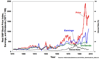
Familiar examples of stochastic processes include stock market and exchange rate fluctuations; signals such as speech; audio and video; medical data such as a patient's EKG, EEG, blood pressure or temperature; and random movement such as Brownian motion or random walks.
A generalization, the random field, is defined by letting the variables be parametrized by members of a topological space instead of time. Examples of random fields include static images, random terrain (landscapes), wind waves and composition variations of a heterogeneous material.
Formal definition and basic properties
Definition
Given a probability space and a measurable space , an S-valued stochastic process is a collection of S-valued random variables on , indexed by a totally ordered set T ("time"). That is, a stochastic process X is a collection


where each is an S-valued random variable on . The space S is then called the state space of the process.

Finite-dimensional distributions
Let X be an S-valued stochastic process. For every finite sequence , the k-tuple is a random variable taking values in . The distribution of this random variable is a probability measure on . This is called a finite-dimensional distribution of X.


Under suitable topological restrictions, a suitably "consistent" collection of finite-dimensional distributions can be used to define a stochastic process (see Kolmogorov extension in the "Construction" section).
History of stochastic processes
Stochastic processes were first studied rigorously in the late 19th century to aid in understanding financial markets and Brownian motion. The first person to describe the mathematics behind Brownian motion was Thorvald N. Thiele in a paper on the method of least squares published in 1880. This was followed independently by Louis Bachelier in 1900 in his PhD thesis "The theory of speculation", in which he presented a stochastic analysis of the stock and option markets. Albert Einstein (in one of his 1905 papers) and Marian Smoluchowski (1906) brought the solution of the problem to the attention of physicists, and presented it as a way to indirectly confirm the existence of atoms and molecules. Their equations describing Brownian motion were subsequently verified by the experimental work of Jean Baptiste Perrin in 1908.
An excerpt from Einstein's paper describes the fundamentals of a stochastic model:
"It must clearly be assumed that each individual particle executes a motion which is independent of the motions of all other particles; it will also be considered that the movements of one and the same particle in different time intervals are independent processes, as long as these time intervals are not chosen too small.
We introduce a time interval into consideration, which is very small compared to the observable time intervals, but nevertheless so large that in two successive time intervals , the motions executed by the particle can be thought of as events which are independent of each other".

Construction
In the ordinary axiomatization of probability theory by means of measure theory, the problem is to construct a sigma-algebra of measurable subsets of the space of all functions, and then put a finite measure on it. For this purpose one traditionally uses a method called Kolmogorov extension.[5]
Kolmogorov extension
The Kolmogorov extension proceeds along the following lines: assuming that a probability measure on the space of all functions exists, then it can be used to specify the joint probability distribution of finite-dimensional random variables . Now, from this n-dimensional probability distribution we can deduce an (n − 1)-dimensional marginal probability distribution for . Note that the obvious compatibility condition, namely, that this marginal probability distribution be in the same class as the one derived from the full-blown stochastic process, is not a requirement. Such a condition only holds, for example, if the stochastic process is a Wiener process (in which case the marginals are all gaussian distributions of the exponential class) but not in general for all stochastic processes. When this condition is expressed in terms of probability densities, the result is called the Chapman–Kolmogorov equation.


The Kolmogorov extension theorem guarantees the existence of a stochastic process with a given family of finite-dimensional probability distributions satisfying the Chapman–Kolmogorov compatibility condition.
Separability, or what the Kolmogorov extension does not provide
Recall that in the Kolmogorov axiomatization, measurable sets are the sets which have a probability or, in other words, the sets corresponding to yes/no questions that have a probabilistic answer.
The Kolmogorov extension starts by declaring to be measurable all sets of functions where finitely many coordinates are restricted to lie in measurable subsets of . In other words, if a yes/no question about f can be answered by looking at the values of at most finitely many coordinates, then it has a probabilistic answer.
![[f(x_{1}),\dots ,f(x_{n})]](../I/m/0039fe22d49daee6eb148604a65805718f5bfef3.svg)

In measure theory, if we have a countably infinite collection of measurable sets, then the union and intersection of all of them is a measurable set. For our purposes, this means that yes/no questions that depend on countably many coordinates have a probabilistic answer.
The good news is that the Kolmogorov extension makes it possible to construct stochastic processes with fairly arbitrary finite-dimensional distributions. Also, every question that one could ask about a sequence has a probabilistic answer when asked of a random sequence. The bad news is that certain questions about functions on a continuous domain don't have a probabilistic answer. One might hope that the questions that depend on uncountably many values of a function be of little interest, but the really bad news is that virtually all concepts of calculus are of this sort. For example:
all require knowledge of uncountably many values of the function.
One solution to this problem is to require that the stochastic process be separable. In other words, that there be some countable set of coordinates whose values determine the whole random function f.

The Kolmogorov continuity theorem guarantees that processes that satisfy certain constraints on the moments of their increments have continuous modifications and are therefore separable.
Filtrations
Given a probability space , a filtration is a weakly increasing collection of sigma-algebras on , , indexed by some totally ordered set , and bounded above by , i.e. for s,t with s < t,


- .

A stochastic process on the same time set is said to be adapted to the filtration if, for every t , is -measurable.[6]


Natural filtration
Given a stochastic process , the natural filtration for (or induced by) this process is the filtration where is generated by all values of up to time s = t, i.e. .


A stochastic process is always adapted to its natural filtration.
Classification
Stochastic processes can be classified according to the cardinality of its index set (usually interpreted as time) and state space.
Discrete time and discrete state space
If both and belong to , the set of natural numbers, then we have models which lead to Markov chains. For example:


(a) If means the bit (0 or 1) in position of a sequence of transmitted bits, then can be modelled as a Markov chain with two states. This leads to the error-correcting Viterbi algorithm in data transmission.
(b) If represents the combined genotype of a breeding couple in the th generation in an inbreeding model, it can be shown that the proportion of heterozygous individuals in the population approaches zero as goes to ∞.[7]
Continuous time and continuous state space
The paradigm of continuous stochastic process is that of the Wiener process. In its original form the problem was concerned with a particle floating on a liquid surface, receiving "kicks" from the molecules of the liquid. The particle is then viewed as being subject to a random force which, since the molecules are very small and very close together, is treated as being continuous and since the particle is constrained to the surface of the liquid by surface tension, is at each point in time a vector parallel to the surface. Thus, the random force is described by a two-component stochastic process; two real-valued random variables are associated to each point in the index set, time, (note that since the liquid is viewed as being homogeneous the force is independent of the spatial coordinates) with the domain of the two random variables being R, giving the x and y components of the force. A treatment of Brownian motion generally also includes the effect of viscosity, resulting in an equation of motion known as the Langevin equation.[8]
Discrete time and continuous state space
If the index set of the process is N (the natural numbers), and the range is R (the real numbers), there are some natural questions to ask about the sample sequences of a process {Xi}i ∈ N, where a sample sequence is {Xi(ω)}i ∈ N.
- What is the probability that each sample sequence is bounded?
- What is the probability that each sample sequence is monotonic?
- What is the probability that each sample sequence has a limit as the index approaches ∞?
- What is the probability that the series obtained from a sample sequence from converges?
- What is the probability distribution of the sum?

Main applications of discrete time continuous state stochastic models include Markov chain Monte Carlo (MCMC) and the analysis of Time Series.
Continuous time and discrete state space
Similarly, if the index space I is a finite or infinite interval, we can ask about the sample paths {Xt(ω)}t ∈ I
- What is the probability that it is bounded/integrable...?
- What is the probability that it has a limit at ∞
- What is the probability distribution of the integral?
See also
- List of stochastic processes topics
- Covariance function
- Dynamics of Markovian particles
- Entropy rate (for a stochastic process)
- Ergodic process
- Gillespie algorithm
- Interacting particle system
- Law (stochastic processes)
- Markov chain
- Probabilistic cellular automaton
- Random field
- Randomness
- Stationary process
- Statistical model
- Stochastic calculus
- Stochastic control
References
- ↑ Dodge, Yadolah (2006). The Oxford Dictionary of Statistical Terms. Oxford, England: Oxford University Press. p. 335. ISBN 9780199206131.
- ↑ Lindsey, J. K. (2004). Statistical Analysis of Stochastic Processes in Time. Cambridge, England: Cambridge University Press. p. 3. ISBN 9780521837415.
- ↑ Lawler, G. (2006). Introduction to Stochastic processes (2 ed.). CRC Press. p. 1.
A stochastic process is a random process evolving with time. More precisely, a stochastic process is a collection of random variables indexed by time.
- ↑ Einstein, Albert (1926). "Investigations on the Theory of the Brownian Movement" (PDF).
- ↑ Karlin, Samuel & Taylor, Howard M. (1998). An Introduction to Stochastic Modeling, Academic Press. ISBN 0-12-684887-4.
- ↑ Durrett, Rick (2010). Probability: Theory and Examples (Fourth ed.). Cambridge: Cambridge University Press. ISBN 978-0-521-76539-8.
- ↑ Allen, Linda J. S., An Introduction to Stochastic Processes with Applications to Biology, 2nd Edition, Chapman and Hall, 2010, ISBN 1-4398-1882-7
- ↑ Gardiner, C. Handbook of Stochastic Methods: for Physics, Chemistry and the Natural Sciences, 3rd ed., Springer, 2004, ISBN 3540208828
Further reading
- Wio, S. Horacio, Deza, R. Roberto & Lopez, M. Juan (2012). An Introduction to Stochastic Processes and Nonequilibrium Statistical Physics. World Scientific Publishing. ISBN 978-981-4374-78-1.
- Papoulis, Athanasios & Pillai, S. Unnikrishna (2001). Probability, Random Variables and Stochastic Processes. McGraw-Hill Science/Engineering/Math. ISBN 0-07-281725-9.
- Boris Tsirelson. "Lecture notes in Advanced probability theory". Archived from the original on November 28, 2008.
- Doob, J. L. (1953). Stochastic Processes. Wiley.
- Klebaner, Fima C. (2011). Introduction to Stochastic Calculus With Applications. Imperial College Press. ISBN 1-84816-831-4.
- Bruce Hajek (July 2006). "An Exploration of Random Processes for Engineers".
- "An 8 foot tall Probability Machine (named Sir Francis) comparing stock market returns to the randomness of the beans dropping through the quincunx pattern". Index Funds Advisors.
- "Popular Stochastic Processes used in Quantitative Finance". sitmo.com.
- "Interactive Web Application: Stochastic Processes used in Quantitative Finance". TuringFinance.com.
- "Addressing Risk and Uncertainty".