Attractor
In the mathematical field of dynamical systems, an attractor is a set of numerical values toward which a system tends to evolve, for a wide variety of starting conditions of the system.[1] System values that get close enough to the attractor values remain close even if slightly disturbed.
In finite-dimensional systems, the evolving variable may be represented algebraically as an n-dimensional vector. The attractor is a region in n-dimensional space. In physical systems, the n dimensions may be, for example, two or three positional coordinates for each of one or more physical entities; in economic systems, they may be separate variables such as the inflation rate and the unemployment rate.
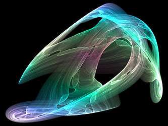
If the evolving variable is two- or three-dimensional, the attractor of the dynamic process can be represented geometrically in two or three dimensions, (as for example in the three-dimensional case depicted to the right). An attractor can be a point, a finite set of points, a curve, a manifold, or even a complicated set with a fractal structure known as a strange attractor (see strange attractor below). If the variable is a scalar, the attractor is a subset of the real number line. Describing the attractors of chaotic dynamical systems has been one of the achievements of chaos theory.
A trajectory of the dynamical system in the attractor does not have to satisfy any special constraints except for remaining on the attractor, forward in time. The trajectory may be periodic or chaotic. If a set of points is periodic or chaotic, but the flow in the neighborhood is away from the set, the set is not an attractor, but instead is called a repeller (or repellor).
Motivation
A dynamical system is generally described by one or more differential or difference equations. The equations of a given dynamical system specify its behavior over any given short period of time. To determine the system's behavior for a longer period, it is often necessary to integrate the equations, either through analytical means or through iteration, often with the aid of computers.
Dynamical systems in the physical world tend to arise from dissipative systems: if it were not for some driving force, the motion would cease. (Dissipation may come from internal friction, thermodynamic losses, or loss of material, among many causes.) The dissipation and the driving force tend to balance, killing off initial transients and settle the system into its typical behavior. The subset of the phase space of the dynamical system corresponding to the typical behavior is the attractor, also known as the attracting section or attractee.
Invariant sets and limit sets are similar to the attractor concept. An invariant set is a set that evolves to itself under the dynamics. Attractors may contain invariant sets. A limit set is a set of points such that there exists some initial state that ends up arbitrarily close to the limit set (i.e. to each point of the set) as time goes to infinity. Attractors are limit sets, but not all limit sets are attractors: It is possible to have some points of a system converge to a limit set, but different points when perturbed slightly off the limit set may get knocked off and never return to the vicinity of the limit set.
For example, the damped pendulum has two invariant points: the point x0 of minimum height and the point x1 of maximum height. The point x0 is also a limit set, as trajectories converge to it; the point x1 is not a limit set. Because of the dissipation due to air resistance, the point x0 is also an attractor. If there was no dissipation, x0 would not be an attractor.
Mathematical definition
Let t represent time and let f(t, •) be a function which specifies the dynamics of the system. That is, if a is an n-dimensional point in the phase space, representing the initial state of the system, then f(0, a) = a and, for a positive value of t, f(t, a) is the result of the evolution of this state after t units of time. For example, if the system describes the evolution of a free particle in one dimension then the phase space is the plane R2 with coordinates (x,v), where x is the position of the particle, v is its velocity, a = (x,v), and the evolution is given by

An attractor is a subset A of the phase space characterized by the following three conditions:
- A is forward invariant under f: if a is an element of A then so is f(t,a), for all t > 0.
- There exists a neighborhood of A, called the basin of attraction for A and denoted B(A), which consists of all points b that "enter A in the limit t → ∞". More formally, B(A) is the set of all points b in the phase space with the following property:
- For any open neighborhood N of A, there is a positive constant T such that f(t,b) ∈ N for all real t > T.
- There is no proper (non-empty) subset of A having the first two properties.
Since the basin of attraction contains an open set containing A, every point that is sufficiently close to A is attracted to A. The definition of an attractor uses a metric on the phase space, but the resulting notion usually depends only on the topology of the phase space. In the case of Rn, the Euclidean norm is typically used.
Many other definitions of attractor occur in the literature. For example, some authors require that an attractor have positive measure (preventing a point from being an attractor), others relax the requirement that B(A) be a neighborhood [2]
Types of attractors
Attractors are portions or subsets of the phase space of a dynamic system. Until the 1960s, attractors were thought of as being simple geometric subsets of the phase space, like points, lines, surfaces, and simple regions of three-dimensional space. More complex attractors that cannot be categorized as simple geometric subsets, such as topologically wild sets, were known of at the time but were thought to be fragile anomalies. Stephen Smale was able to show that his horseshoe map was robust and that its attractor had the structure of a Cantor set.
Two simple attractors are a fixed point and the limit cycle. Attractors can take on many other geometric shapes (phase space subsets). But when these sets (or the motions within them) cannot be easily described as simple combinations (e.g. intersection and union) of fundamental geometric objects (e.g. lines, surfaces, spheres, toroids, manifolds), then the attractor is called a strange attractor.
Fixed point
A fixed point of a function or transformation is a point that is mapped to itself by the function or transformation.[1] If we regard the evolution of a dynamical system as a series of transformations, then there may or may not be a point which remains fixed under each transformation. The final state that a dynamical system evolves towards corresponds to an attracting fixed point of the evolution function for that system, such as the center bottom position of a damped pendulum, the level and flat water line of sloshing water in a glass, or the bottom center of a bowl contain a rolling marble. But the fixed point(s) of a dynamic system is not necessarily an attractor of the system. For example, if the bowl containing a rolling marble was inverted and the marble was balanced on top of the bowl, the center bottom (now top) of the bowl is a fixed state, but not an attractor. This is equivalent to the difference between stable and unstable equilibria. In the case of a marble on top of an inverted bowl (a hill), that point at the top of the bowl (hill) is a fixed point (equilibrium), but not an attractor (stable equilibrium).
In addition, physical dynamic systems with at least one fixed point invariably have multiple fixed points and attractors due to the reality of dynamics in the physical world, including the nonlinear dynamics of stiction, friction, surface roughness, deformation (both elastic and plasticity), and even quantum mechanics.[3] In the case of a marble on top of an inverted bowl, even if the bowl seems perfectly hemispherical, and the marble's spherical shape, are both much more complex surfaces when examined under a microscope, and their shapes change or deform during contact. Any physical surface can be seen to have a rough terrain of multiple peaks, valleys, saddle points, ridges, ravines, and plains.[4] There are many points in this surface terrain (and the dynamic system of a similarly rough marble rolling around on this microscopic terrain) that are considered stationary or fixed points, some of which are categorized as attractors.
Finite number of points
In a discrete-time system, an attractor can take the form of a finite number of points that are visited in sequence. Each of these points is called a periodic point. This is illustrated by the logistic map, which depending on its specific parameter value can have an attractor consisting of 2n points, 3×2n points, etc., for any value of n.
Limit cycle
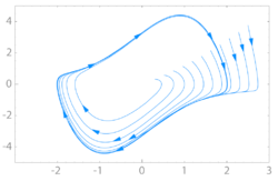
A limit cycle is a periodic orbit of a continuous dynamical system that is isolated. Examples include the swings of a pendulum clock, the tuning circuit of a radio, and the heartbeat while resting. (The limit cycle of an ideal pendulum is not an example of a limit cycle attractor because its orbits are not isolated: in the phase space of the ideal pendulum, near any point of a periodic orbit there is another point that belongs to a different periodic orbit, so the former orbit is not attracting).
Limit torus
There may be more than one frequency in the periodic trajectory of the system through the state of a limit cycle. For example, in physics, one frequency may dictate the rate at which a planet orbits a star while a second frequency describes the oscillations in the distance between the two bodies. If two of these frequencies form an irrational fraction (i.e. they are incommensurate), the trajectory is no longer closed, and the limit cycle becomes a limit torus. This kind of attractor is called an Nt-torus if there are Nt incommensurate frequencies. For example, here is a 2-torus:
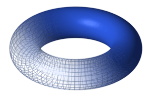
A time series corresponding to this attractor is a quasiperiodic series: A discretely sampled sum of Nt periodic functions (not necessarily sine waves) with incommensurate frequencies. Such a time series does not have a strict periodicity, but its power spectrum still consists only of sharp lines.
Strange attractor
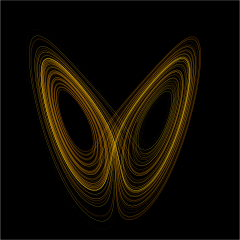
An attractor is called strange if it has a fractal structure.[1] This is often the case when the dynamics on it are chaotic, but strange nonchaotic attractors also exist. If a strange attractor is chaotic, exhibiting sensitive dependence on initial conditions, then any two arbitrarily close alternative initial points on the attractor, after any of various numbers of iterations, will lead to points that are arbitrarily far apart (subject to the confines of the attractor), and after any of various other numbers of iterations will lead to points that are arbitrarily close together. Thus a dynamic system with a chaotic attractor is locally unstable yet globally stable: once some sequences have entered the attractor, nearby points diverge from one another but never depart from the attractor.[5]
The term strange attractor was coined by David Ruelle and Floris Takens to describe the attractor resulting from a series of bifurcations of a system describing fluid flow.[6] Strange attractors are often differentiable in a few directions, but some are like a Cantor dust, and therefore not differentiable. Strange attractors may also be found in presence of noise, where they may be shown to support invariant random probability measures of Sinai–Ruelle–Bowen type.[7]
Examples of strange attractors include the double-scroll attractor, Hénon attractor, Rössler attractor, Tamari attractor, and the Lorenz attractor.
Effect of parameters on the attractor
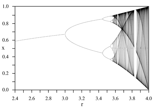
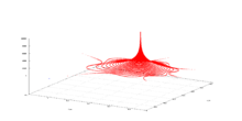
A particular functional form of a dynamic equation can have various types of attractor depending on the particular parameter values used in the function. An example is the well-studied logistic map, whose basins of attraction for various values of the parameter r are shown in the diagram. At some values of the parameter the attractor is a single point, at others it is two points that are visited in turn, at others it is 2n points or k × 2n points that are visited in turn, for any value of n depending on the value of the parameter r, and at other values of r an infinitude of points are visited.[1]

Basins of attraction
An attractor's basin of attraction is the region of the phase space, over which iterations are defined, such that any point (any initial condition) in that region will eventually be iterated into the attractor.[1] For a stable linear system, every point in the phase space is in the basin of attraction. However, in nonlinear systems, some points may map directly or asymptotically to infinity, while other points may lie in a different basin of attraction and map asymptotically into a different attractor; other initial conditions may be in or map directly into a non-attracting point or cycle.
Linear equation or system
A single-variable (univariate) linear difference equation of the homogeneous form diverges to infinity if |a| > 1 from all initial points except 0; there is no attractor and therefore no basin of attraction. But if |a| < 1 all points on the number line map asymptotically (or directly in the case of 0) to 0; 0 is the attractor, and the entire number line is the basin of attraction.

Likewise, a linear matrix difference equation in a dynamic vector X, of the homogeneous form in terms of square matrix A will have all elements of the dynamic vector diverge to infinity if the largest eigenvalue of A is greater than 1 in absolute value; there is no attractor and no basin of attraction. But if the largest eigenvalue is less than 1 in magnitude, all initial vectors will asymptotically converge to the zero vector, which is the attractor; the entire n-dimensional space of potential initial vectors is the basin of attraction.

Similar features apply to linear differential equations. The scalar equation causes all initial values of x except zero to diverge to infinity if a > 0 but to converge to an attractor at the value 0 if a < 0, making the entire number line the basin of attraction for 0. And the matrix system gives divergence from all initial points except the vector of zeroes if any eigenvalue of the matrix A is positive; but if all the eigenvalues are negative the vector of zeroes is an attractor whose basin of attraction is the entire phase space.


Nonlinear equation or system
Equations or systems that are nonlinear can give rise to a richer variety of behavior than can linear systems. One example is Newton's method of iterating to a root of a nonlinear expression. If the expression has more than one real root, some starting points for the iterative algorithm will lead to one of the roots asymptotically, and other starting points will lead to another. The basins of attraction for the expression's roots are generally not simple—it is not simply that the points nearest one root all map there, giving a basin of attraction consisting of nearby points. The basins of attraction can be infinite in number and arbitrarily small. For example,[8] for the function , the following initial conditions are in successive basins of attraction:


- 2.35287527 converges to 4;
- 2.35284172 converges to −3;
- 2.35283735 converges to 4;
- 2.352836327 converges to −3;
- 2.352836323 converges to 1.
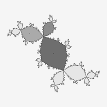
Newton's method can also be applied to complex functions to find their roots. Each root has a basin of attraction in the complex plane; these basins can be mapped as in the image shown. As can be seen, the combined basin of attraction for a particular root can have many disconnected regions. For many complex functions, the boundaries of the basins of attraction are fractals.
Partial differential equations
Parabolic partial differential equations may have finite-dimensional attractors. The diffusive part of the equation damps higher frequencies and in some cases leads to a global attractor. The Ginzburg–Landau, the Kuramoto–Sivashinsky, and the two-dimensional, forced Navier–Stokes equations are all known to have global attractors of finite dimension.
For the three-dimensional, incompressible Navier–Stokes equation with periodic boundary conditions, if it has a global attractor, then this attractor will be of finite dimensions.
Numerical localization (visualization) of attractors: self-excited and hidden attractors
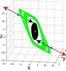
From a computational point of view, attractors can be naturally regarded as self-excited attractors or hidden attractors.[9][10][11][12] Self-excited attractors can be localized numerically by standard computational procedures, in which after a transient sequence, a trajectory starting from a point on an unstable manifold in a small neighborhood of an unstable equilibrium reaches an attractor (like classical attractors in the Van der Pol, Belousov–Zhabotinsky, Lorenz, and many other dynamical systems). In contrast, the basin of attraction of a hidden attractor does not contain neighborhoods of equilibria, so the hidden attractor cannot be localized by standard computational procedures.
See also
| Wikimedia Commons has media related to Attractor. |
References
- 1 2 3 4 5 Boeing, G. (2016). "Visual Analysis of Nonlinear Dynamical Systems: Chaos, Fractals, Self-Similarity and the Limits of Prediction". Systems. 4 (4): 37. doi:10.3390/systems4040037. Retrieved 2016-12-02.
- ↑ Milnor, J. (1985). "On the Concept of Attractor." Comm. Math. Phys 99: 177–195.
- ↑ Greenwood, J. A.; J. B. P. Williamson (6 December 1966). "Contact of Nominally Flat Surfaces". Proceedings of the Royal Society. 295 (1442): 300–319. doi:10.1098/rspa.1966.0242. Retrieved 31 March 2013.
- ↑ Vorberger, T. V. (1990). Surface Finish Metrology Tutorial (PDF). U.S. Department of Commerce, National Institute of Standards (NIST). p. 5.
- ↑ Grebogi, Celso, Edward Ott, and James A. Yorke. "Chaos, Strange Attractors, and Fractal Basin Boundaries in Nonlinear Dynamics." Science 238, no. 4827 (1987): 632–638.
- ↑ Ruelle, David; Takens, Floris (1971). "On the nature of turbulence". Communications in Mathematical Physics. 20 (3): 167–192. doi:10.1007/bf01646553.
- ↑ Chekroun M. D.; Simonnet E. & Ghil M. (2011). "Stochastic climate dynamics: Random attractors and time-dependent invariant measures". Physica D. 240 (21): 1685–1700. doi:10.1016/j.physd.2011.06.005.
- ↑ Dence, Thomas, "Cubics, chaos and Newton's method", Mathematical Gazette 81, November 1997, 403–408.
- ↑ Leonov G.A.; Vagaitsev V.I.; Kuznetsov N.V. (2011). "Localization of hidden Chua's attractors" (PDF). Physics Letters A. 375 (23): 2230–2233. doi:10.1016/j.physleta.2011.04.037.
- ↑ Bragin V.O.; Vagaitsev V.I.; Kuznetsov N.V.; Leonov G.A. (2011). "Algorithms for Finding Hidden Oscillations in Nonlinear Systems. The Aizerman and Kalman Conjectures and Chua's Circuits" (PDF). Journal of Computer and Systems Sciences International. 50 (5): 511–543. doi:10.1134/S106423071104006X.
- ↑ Leonov G.A.; Vagaitsev V.I.; Kuznetsov N.V. (2012). "Hidden attractor in smooth Chua systems" (PDF). Physica D. 241 (18): 1482–1486. doi:10.1016/j.physd.2012.05.016.
- ↑ Leonov G.A.; Kuznetsov N.V. (2013). "Hidden attractors in dynamical systems. From hidden oscillations in Hilbert–Kolmogorov, Aizerman, and Kalman problems to hidden chaotic attractor in Chua circuits". International Journal of Bifurcation and Chaos. 23 (1): art. no. 1330002. doi:10.1142/S0218127413300024.
Further reading
- John Milnor (ed.). "Attractor". Scholarpedia.
- David Ruelle; Floris Takens (1971). "On the nature of turbulence". Communications of Mathematical Physics. 20 (3): 167–192. doi:10.1007/BF01646553.
- D. Ruelle (1981). "Small random perturbations of dynamical systems and the definition of attractors". Communications of Mathematical Physics. 82: 137–151. doi:10.1007/BF01206949.
- John Milnor (1985). "On the concept of attractor". Communications of Mathematical Physics. 99 (2): 177–195. doi:10.1007/BF01212280.
- David Ruelle (1989). Elements of Differentiable Dynamics and Bifurcation Theory. Academic Press. ISBN 0-12-601710-7.
- Ruelle, David (August 2006). "What is...a Strange Attractor?" (PDF). Notices of the American Mathematical Society. 53 (7): 764–765. Retrieved 16 January 2008.
- Grebogi; Ott; Pelikan; Yorke (1984). "Strange attractors that are not chaotic". Physica D. 13: 261–268. doi:10.1016/0167-2789(84)90282-3.
- Chekroun, M. D.; E. Simonnet; M. Ghil (2011). "Stochastic climate dynamics: Random attractors and time-dependent invariant measures". Physica D. 240 (21): 1685–1700. doi:10.1016/j.physd.2011.06.005.
- Edward N. Lorenz (1996) The Essence of Chaos ISBN 0-295-97514-8
- James Gleick (1988) Chaos: Making a New Science ISBN 0-14-009250-1
External links
- Basin of attraction on Scholarpedia
- A gallery of trigonometric strange attractors
- Double scroll attractor Chua's circuit simulation
- A gallery of polynomial strange attractors
- Chaoscope, a 3D Strange Attractor rendering freeware
- Research abstract and software laboratory
- Online strange attractors generator
- Interactive trigonometric attractors generator
- Economic attractor