Linear least squares (mathematics)
| Part of a series on Statistics |
| Regression analysis |
|---|
 |
| Models |
| Estimation |
| Background |
|
In statistics and mathematics, linear least squares is an approach fitting a mathematical or statistical model to data in cases where the idealized value provided by the model for any data point is expressed linearly in terms of the unknown parameters of the model. The resulting fitted model can be used to summarize the data, to predict unobserved values from the same system, and to understand the mechanisms that may underlie the system.
Mathematically, linear least squares is the problem of approximately solving an overdetermined system of linear equations, where the best approximation is defined as that which minimizes the sum of squared differences between the data values and their corresponding modeled values. The approach is called linear least squares since the assumed function is linear in the parameters to be estimated. Linear least squares problems are convex and have a closed-form solution that is unique, provided that the number of data points used for fitting equals or exceeds the number of unknown parameters, except in special degenerate situations. In contrast, non-linear least squares problems generally must be solved by an iterative procedure, and the problems can be non-convex with multiple optima for the objective function. If prior distributions are available, then even an underdetermined system can be solved using the Bayesian MMSE estimator.
In statistics, linear least squares problems correspond to a particularly important type of statistical model called linear regression which arises as a particular form of regression analysis. One basic form of such a model is an ordinary least squares model. The present article concentrates on the mathematical aspects of linear least squares problems, with discussion of the formulation and interpretation of statistical regression models and statistical inferences related to these being dealt with in the articles just mentioned. See outline of regression analysis for an outline of the topic.
Example
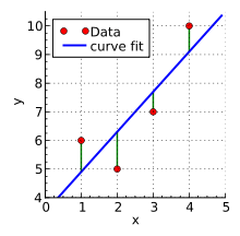
As a result of an experiment, four data points were obtained, and (shown in red in the picture on the right). We hope to find a line that best fits these four points. In other words, we would like to find the numbers and that approximately solve the overdetermined linear system


of four equations in two unknowns in some "best" sense.
The "error", at each point, between the curve fit and the data is the difference between the right- and left-hand sides of the equations above. The least squares approach to solving this problem is to try to make the sum of the squares of these errors as small as possible; that is, to find the minimum of the function
![{\begin{aligned}S(\beta _{1},\beta _{2})=&\left[6-(\beta _{1}+1\beta _{2})\right]^{2}+\left[5-(\beta _{1}+2\beta _{2})\right]^{2}\\&+\left[7-(\beta _{1}+3\beta _{2})\right]^{2}+\left[10-(\beta _{1}+4\beta _{2})\right]^{2}\\&=4\beta _{1}^{2}+30\beta _{2}^{2}+20\beta _{1}\beta _{2}-56\beta _{1}-154\beta _{2}+210.\end{aligned}}](../I/m/b4ce34fff67196dcbef77b2de4daf415f95244b0.svg)
The minimum is determined by calculating the partial derivatives of with respect to and and setting them to zero


This results in a system of two equations in two unknowns, called the normal equations, which give, when solved


and the equation of the line of best fit. The residuals, that is, the discrepancies between the values from the experiment and the values calculated using the line of best fit are then found to be and (see the picture on the right). The minimum value of the sum of squares of the residuals is


More generally, one can have regressors , and a linear model


- .

Using a quadratic model


Importantly, in "linear least squares", we are not restricted to using a line as the model as in the above example. For instance, we could have chosen the restricted quadratic model . This model is still linear in the parameter, so we can still perform the same analysis, constructing a system of equations from the data points:


The partial derivatives with respect to the parameters (this time there is only one) are again computed and set to 0:

and solved

leading to the resulting best fit model

The general problem
Consider an overdetermined system

of m linear equations in n unknown coefficients, β1,β2,…,βn, with m > n. (Note: for a linear model as above, not all of contains information on the data points. The first column is populated with ones, , only the other columns contain actual data, and n = number of regressors + 1). This can be written in matrix form as


where

Such a system usually has no solution, so the goal is instead to find the coefficients which fit the equations "best," in the sense of solving the quadratic minimization problem


where the objective function S is given by

A justification for choosing this criterion is given in properties below. This minimization problem has a unique solution, provided that the n columns of the matrix are linearly independent, given by solving the normal equations


The matrix is known as the Gramian matrix of , which possesses several nice properties such as being a positive semi-definite matrix, and the matrix is known as the moment matrix of regressand by regressors.[1] Finally, is the coefficient vector of the least-squares hyperplane, expressed as


Example implementation
MATLAB
The following MATLAB code shows implementation of this approach on the data used in the first example above.
% MATLAB code for finding the best fit line using least squares method
input = [...                 % input in the form of matrix
    1, 6;...                 % rows contain points
    2, 5;...
    3, 7;...
    4, 10];
m = length(input);             % number of points
X = [ones(m,1), input(:,1)];   % forming X of X beta = y
y = input(:,2);                % forming y of X beta = y
betaHat = (X' * X) \ X' * y;   % computing projection of matrix X on y, giving beta
% display best fit parameters
disp(betaHat);
% plot the best fit line
xx = linspace(0, 5, 2);
yy = betaHat(1) + betaHat(2)*xx;
plot(xx, yy)
% plot the points (data) for which we found the best fit
hold on
plot(input(:,1), input(:,2), 'or')
hold off
Python
Python code using the same variable naming as the MATLAB code above:
import numpy as np
import matplotlib.pyplot as plt
input = np.array([
    [1, 6],
    [2, 5],
    [3, 7],
    [4, 10]
])
m = np.shape(input)[0]
X = np.matrix([np.ones(m), input[:,0]]).T
y = np.matrix(input[:,1]).T
betaHat = np.linalg.inv(X.T.dot(X)).dot(X.T).dot(y)
print(betaHat)
plt.figure(1)
xx = np.linspace(0, 5, 2)
yy = np.array(betaHat[0] + betaHat[1] * xx)
plt.plot(xx, yy.T, color='b')
plt.scatter(input[:,0], input[:,1], color='r')
plt.show()
Julia (programming language)
using Plots
pyplot() #choose plotting backend
input = [
    1 6
    2 5
    3 7
    4 10]
m = size(input)[1]
X = [ones(m) input[:,1]]
y = input[:,2]
betaHat = (X' * X ) \ X' * y #backslash computes LS-solution as in Matlab
print(betaHat)
plot(x->betaHat[2]*x + betaHat[1],0,5,label="curve fit")
scatter!(input[:,1],input[:,2],label="data")
R (programming language)
m <- 4
n <- 2
input <- matrix(c(1, 6, 2, 5, 3, 7, 4, 10), ncol = n, byrow = T)
k <- rep(1,m)
X <- cbind(k, input[,1])
y <- input[,2]
X.T <- t(X)
betaHat <- solve(X.T%*%X) %*% X.T %*%y
print(betaHat)
plot(input)
abline(betaHat[1], betaHat[2])
Derivation of the normal equations
Define the th residual to be

- .

Then can be rewritten


Given that S is convex, it is minimized when its gradient vector is zero (This follows by definition: if the gradient vector is not zero, there is a direction in which we can move to minimize it further - see maxima and minima.) The elements of the gradient vector are the partial derivatives of S with respect to the parameters:

The derivatives are

Substitution of the expressions for the residuals and the derivatives into the gradient equations gives

Thus if minimizes S, we have


Upon rearrangement, we obtain the normal equations:

The normal equations are written in matrix notation as
- (where XT is the matrix transpose of X).

The solution of the normal equations yields the vector of the optimal parameter values.
Derivation directly in terms of matrices
The normal equations can be derived directly from a matrix representation of the problem as follows. The objective is to minimize

Note that : has the dimension 1x1 (the number of columns of ), so it is a scalar and equal to its own transpose, hence and the quantity to minimize becomes


Differentiating this with respect to and equating to zero to satisfy the first-order conditions gives

which is equivalent to the above-given normal equations. A sufficient condition for satisfaction of the second-order conditions for a minimum is that have full column rank, in which case is positive definite.
Derivation without calculus
When is positive definite, the formula for the minimizing value of can be derived without the use of derivatives. The quantity

can be written as

where depends only on and , and is the inner product defined by


It follows that is equal to


and therefore minimized exactly when

Generalization for complex equations
In general, the coefficients of the matrices and can be complex. By using a Hermitian transpose instead of a simple transpose, it is possible to find a vector which minimize , just as for the real matrices. In order to get the normal equations we follow a similar path as in previous derivations:


where stands for Hermitian transpose.

We should now take derivatives of with respect to each of the coefficient , but first we separate real and imaginary part to deal with the conjugate factors in above expression. For the we have


and the derivatives changes into

After rewriting in the summation form and writing explicite, we can calculate both partial derivatives with result:


which, after adding it together and comparing to zero ( minimalization condition for ) yields

In matrix form:

Computation
A general approach to the least squares problem can be described as follows. Suppose that we can find an n by m matrix S such that XS is an orthogonal projection onto the image of X. Then a solution to our minimization problem is given by


simply because

is exactly a sought for orthogonal projection of onto an image of X (see the picture below and note that as explained in the next section the image of X is just a subspace generated by column vectors of X). A few popular ways to find such a matrix S are described below.
Inverting the matrix of the normal equations
The algebraic solution of the normal equations can be written as

where X + is the Moore–Penrose pseudoinverse of X. Although this equation is correct, and can work in many applications, it is not computationally efficient to invert the normal equations matrix (the Gramian matrix). An exception occurs in numerical smoothing and differentiation where an analytical expression is required.
If the matrix XTX is well-conditioned and positive definite, implying that it has full rank, the normal equations can be solved directly by using the Cholesky decomposition RTR, where R is an upper triangular matrix, giving:

The solution is obtained in two stages, a forward substitution step, solving for z:

followed by a backward substitution, solving for

Both substitutions are facilitated by the triangular nature of R.
See example of linear regression for a worked-out numerical example with three parameters.
Orthogonal decomposition methods
Orthogonal decomposition methods of solving the least squares problem are slower than the normal equations method but are more numerically stable because they avoid forming the product XTX.
The residuals are written in matrix notation as

The matrix X is subjected to an orthogonal decomposition, e.g., the QR decomposition as follows.
- ,

where Q is an m×m orthogonal matrix (QTQ=I) and R is an n×n upper triangular matrix with .

The residual vector is left-multiplied by QT.

Because Q is orthogonal, the sum of squares of the residuals, s, may be written as:

Since v doesn't depend on β, the minimum value of s is attained when the upper block, u, is zero. Therefore the parameters are found by solving:

These equations are easily solved as R is upper triangular.
An alternative decomposition of X is the singular value decomposition (SVD)[2]
- ,

where U is m by m orthogonal matrix, V is n by n orthogonal matrix and is an m by n matrix with all its elements outside of the main diagonal equal to 0. The pseudoinverse of is easily obtained by inverting its non-zero diagonal elements and transposing. Hence,


where P is obtained from by replacing its non-zero diagonal elements with ones. Since (the property of pseudoinverse), the matrix is an orthogonal projection onto the image (column-space) of X. In accordance with a general approach described in the introduction above (find XS which is an orthogonal projection),


- ,

and thus,

is a solution of a least squares problem. This method is the most computationally intensive, but is particularly useful if the normal equations matrix, XTX, is very ill-conditioned (i.e. if its condition number multiplied by the machine's relative round-off error is appreciably large). In that case, including the smallest singular values in the inversion merely adds numerical noise to the solution. This can be cured with the truncated SVD approach, giving a more stable and exact answer, by explicitly setting to zero all singular values below a certain threshold and so ignoring them, a process closely related to factor analysis.
Properties of the least-squares estimators


The gradient equations at the minimum can be written as

A geometrical interpretation of these equations is that the vector of residuals, is orthogonal to the column space of X, since the dot product is equal to zero for any conformal vector, v. This means that is the shortest of all possible vectors , that is, the variance of the residuals is the minimum possible. This is illustrated at the right.


Introducing and a matrix K with the assumption that a matrix is non-singular and KT X = 0 (cf. Orthogonal projections), the residual vector should satisfy the following equation:

![[X\ K]](../I/m/b0c7583e31f8e4111806d1612b81b39d3f76af01.svg)

The equation and solution of linear least squares are thus described as follows:


If the experimental errors, , are uncorrelated, have a mean of zero and a constant variance, , the Gauss-Markov theorem states that the least-squares estimator, , has the minimum variance of all estimators that are linear combinations of the observations. In this sense it is the best, or optimal, estimator of the parameters. Note particularly that this property is independent of the statistical distribution function of the errors. In other words, the distribution function of the errors need not be a normal distribution. However, for some probability distributions, there is no guarantee that the least-squares solution is even possible given the observations; still, in such cases it is the best estimator that is both linear and unbiased.


For example, it is easy to show that the arithmetic mean of a set of measurements of a quantity is the least-squares estimator of the value of that quantity. If the conditions of the Gauss-Markov theorem apply, the arithmetic mean is optimal, whatever the distribution of errors of the measurements might be.
However, in the case that the experimental errors do belong to a normal distribution, the least-squares estimator is also a maximum likelihood estimator.[3]
These properties underpin the use of the method of least squares for all types of data fitting, even when the assumptions are not strictly valid.
Limitations
An assumption underlying the treatment given above is that the independent variable, x, is free of error. In practice, the errors on the measurements of the independent variable are usually much smaller than the errors on the dependent variable and can therefore be ignored. When this is not the case, total least squares or more generally errors-in-variables models, or rigorous least squares, should be used. This can be done by adjusting the weighting scheme to take into account errors on both the dependent and independent variables and then following the standard procedure.[4][5]
In some cases the (weighted) normal equations matrix XTX is ill-conditioned. When fitting polynomials the normal equations matrix is a Vandermonde matrix. Vandermonde matrices become increasingly ill-conditioned as the order of the matrix increases. In these cases, the least squares estimate amplifies the measurement noise and may be grossly inaccurate. Various regularization techniques can be applied in such cases, the most common of which is called ridge regression. If further information about the parameters is known, for example, a range of possible values of , then various techniques can be used to increase the stability of the solution. For example, see constrained least squares.

Another drawback of the least squares estimator is the fact that the norm of the residuals, is minimized, whereas in some cases one is truly interested in obtaining small error in the parameter , e.g., a small value of . However, since the true parameter is necessarily unknown, this quantity cannot be directly minimized. If a prior probability on is known, then a Bayes estimator can be used to minimize the mean squared error, . The least squares method is often applied when no prior is known. Surprisingly, when several parameters are being estimated jointly, better estimators can be constructed, an effect known as Stein's phenomenon. For example, if the measurement error is Gaussian, several estimators are known which dominate, or outperform, the least squares technique; the best known of these is the James–Stein estimator. This is an example of more general shrinkage estimators that have been applied to regression problems.


Weighted linear least squares
In some cases the observations may be weighted—for example, they may not be equally reliable. In this case, one can minimize the weighted sum of squares:

where wi > 0 is the weight of the ith observation, and W is the diagonal matrix of such weights.
The weights should, ideally, be equal to the reciprocal of the variance of the measurement.[6][7] The normal equations are then:

This method is used in iteratively reweighted least squares.
Parameter errors and correlation
The estimated parameter values are linear combinations of the observed values

Therefore an expression for the residuals (i.e., the estimated errors in the parameters) can be obtained by error propagation from the errors in the observations. Let the variance-covariance matrix for the observations be denoted by M and that of the parameters by Mβ. Then,

When W = M −1 this simplifies to

When unit weights are used (W = I, the identity matrix) it is implied that the experimental errors are uncorrelated and all equal: M = σ2I, where σ2 is the a priori variance of an observation. In any case, σ2 is approximated by the reduced chi-squared :

- ,


where S is the minimum value of the (weighted) objective function:

The denominator, is the number of degrees of freedom; see effective degrees of freedom for generalizations for the case of correlated observations.

In all cases, the variance of the parameter is given by and the covariance between parameters and is given by . Standard deviation is the square root of variance, and the correlation coefficient is given by . These error estimates reflect only random errors in the measurements. The true uncertainty in the parameters is larger due to the presence of systematic errors which, by definition, cannot be quantified. Note that even though the observations may be un-correlated, the parameters are typically correlated.


Parameter confidence limits
It is often assumed, for want of any concrete evidence but often appealing to the central limit theorem—see Normal distribution#Occurrence—that the error on each observation belongs to a normal distribution with a mean of zero and standard deviation . Under that assumption the following probabilities can be derived for a single scalar parameter estimate in terms of its estimated standard error (given here):

- 68% that the interval encompasses the true coefficient value
- 95% that the interval encompasses the true coefficient value
- 99% that the interval encompasses the true coefficient value


The assumption is not unreasonable when m >> n. If the experimental errors are normally distributed the parameters will belong to a Student's t-distribution with m − n degrees of freedom. When m >> n Student's t-distribution approximates a normal distribution. Note, however, that these confidence limits cannot take systematic error into account. Also, parameter errors should be quoted to one significant figure only, as they are subject to sampling error.[8]
When the number of observations is relatively small, Chebychev's inequality can be used for an upper bound on probabilities, regardless of any assumptions about the distribution of experimental errors: the maximum probabilities that a parameter will be more than 1, 2 or 3 standard deviations away from its expectation value are 100%, 25% and 11% respectively.
Residual values and correlation
The residuals are related to the observations by

where H is the idempotent matrix known as the hat matrix:

and I is the identity matrix. The variance-covariance matrix of the residuals, Mr is given by

Thus the residuals are correlated, even if the observations are not.
When ,


The sum of residual values is equal to zero whenever the model function contains a constant term. Left-multiply the expression for the residuals by XT:

Say, for example, that the first term of the model is a constant, so that for all i. In that case it follows that

Thus, in the motivational example, above, the fact that the sum of residual values is equal to zero it is not accidental but is a consequence of the presence of the constant term, α, in the model.
If experimental error follows a normal distribution, then, because of the linear relationship between residuals and observations, so should residuals,[9] but since the observations are only a sample of the population of all possible observations, the residuals should belong to a Student's t-distribution. Studentized residuals are useful in making a statistical test for an outlier when a particular residual appears to be excessively large.
Objective function
The optimal value of the objective function, found by substituting in the optimal expression for the coefficient vector, can be written as (assuming unweighted observations)

the latter equality holding since (I – H) is symmetric and idempotent. It can be shown from this[10] that under an appropriate assignment of weights the expected value of S is m-n. If instead unit weights are assumed, the expected value of S is , where is the variance of each observation.


If it is assumed that the residuals belong to a normal distribution, the objective function, being a sum of weighted squared residuals, will belong to a chi-squared () distribution with m-n degrees of freedom. Some illustrative percentile values of are given in the following table.[11]


These values can be used for a statistical criterion as to the goodness-of-fit. When unit weights are used, the numbers should be divided by the variance of an observation.
Constrained linear least squares
Often it is of interest to solve a linear least squares problem with an additional constraint on the solution. With constrained linear least squares, the original equation

must be fit as closely as possible (in the least squares sense) while ensuring that some other property of is maintained. There are often special purpose algorithms for solving such problems efficiently. Some examples of constraints are given below:
- Equality constrained least squares: the elements of must exactly satisfy (see Ordinary least squares#Constrained estimation.)
- Regularized least squares: the elements of must satisfy
- Non-negative least squares (NNLS): The vector must satisfy the vector inequality defined componentwise—that is, each component must be either positive or zero.
- Box-constrained least squares: The vector must satisfy the vector inequalities , each of which is defined componentwise.
- Integer constrained least squares: all elements of must be integers (instead of real numbers).
- Phase constrained least squares: all elements of must have the same phase (or must be real rather than complex numbers, i.e. phase = 0).


When the constraint only applies to some of the variables, the mixed problem may be solved using separable least squares by letting and represent the unconstrained (1) and constrained (2) components. Then substituting the least squares solution for , i.e.
![\mathbf {X} =[\mathbf {X_{1}} \mathbf {X_{2}} ]](../I/m/a1667b3d53538de2884a4287f8d0aa55ec000d49.svg)
![\mathbf {\beta } ^{\rm {T}}=[\mathbf {\beta _{1}} ^{\rm {T}}\mathbf {\beta _{2}} ^{\rm {T}}]](../I/m/ac2ba398e1eb67bf2ffc15d36acda38064ce73b2.svg)


back into the original expression gives (following some rearrangement) an equation that can be solved as a purely constrained problem in .


where is a projection matrix. Following the constrained estimation of the vector is obtained from the expression above.


Typical uses and applications
- Polynomial fitting: models are polynomials in an independent variable, x:
- Straight line: .[12]
- Quadratic: .
- Cubic, quartic and higher polynomials. For regression with high-order polynomials, the use of orthogonal polynomials is recommended.[13]
- Numerical smoothing and differentiation — this is an application of polynomial fitting.
- Multinomials in more than one independent variable, including surface fitting
- Curve fitting with B-splines [4]
- Chemometrics, Calibration curve, Standard addition, Gran plot, analysis of mixtures


Uses in data fitting
The primary application of linear least squares is in data fitting. Given a set of m data points consisting of experimentally measured values taken at m values of an independent variable ( may be scalar or vector quantities), and given a model function with it is desired to find the parameters such that the model function "best" fits the data. In linear least squares, linearity is meant to be with respect to parameters so


Here, the functions may be nonlinear with respect to the variable x.

Ideally, the model function fits the data exactly, so

for all This is usually not possible in practice, as there are more data points than there are parameters to be determined. The approach chosen then is to find the minimal possible value of the sum of squares of the residuals


so to minimize the function

After substituting for and then for , this minimization problem becomes the quadratic minimization problem above with


and the best fit can be found by solving the normal equations.
Further discussion
The numerical methods for linear least squares are important because linear regression models are among the most important types of model, both as formal statistical models and for exploration of data-sets. The majority of statistical computer packages contain facilities for regression analysis that make use of linear least squares computations. Hence it is appropriate that considerable effort has been devoted to the task of ensuring that these computations are undertaken efficiently and with due regard to round-off error.
Individual statistical analyses are seldom undertaken in isolation, but rather are part of a sequence of investigatory steps. Some of the topics involved in considering numerical methods for linear least squares relate to this point. Thus important topics can be
- Computations where a number of similar, and often nested, models are considered for the same data-set. That is, where models with the same dependent variable but different sets of independent variables are to be considered, for essentially the same set of data-points.
- Computations for analyses that occur in a sequence, as the number of data-points increases.
- Special considerations for very extensive data-sets.
Fitting of linear models by least squares often, but not always, arise in the context of statistical analysis. It can therefore be important that considerations of computation efficiency for such problems extend to all of the auxiliary quantities required for such analyses, and are not restricted to the formal solution of the linear least squares problem.
Rounding errors
Matrix calculations, like any other, are affected by rounding errors. An early summary of these effects, regarding the choice of computation methods for matrix inversion, was provided by Wilkinson.[14]
See also
- Line-line intersection#Nearest point to non-intersecting lines, an application
References
- ↑ Goldberger, Arthur S. (1964). "Classical Linear Regression". Econometric Theory. New York: John Wiley & Sons. pp. 156–212 [p. 158]. ISBN 0-471-31101-4.
- ↑ Lawson, C. L.; Hanson, R. J. (1974). Solving Least Squares Problems. Englewood Cliffs, NJ: Prentice-Hall. ISBN 0-13-822585-0.
- ↑ Margenau, Henry; Murphy, George Moseley (1956). The Mathematics of Physics and Chemistry. Princeton: Van Nostrand.
- 1 2 Gans, Peter (1992). Data fitting in the Chemical Sciences. New York: Wiley. ISBN 0-471-93412-7.
- ↑ Deming, W. E. (1943). Statistical adjustment of Data. New York: Wiley.
- ↑ This implies that the observations are uncorrelated. If the observations are correlated, the expression applies. In this case the weight matrix should ideally be equal to the inverse of the variance-covariance matrix of the observations.
- ↑ Strutz, T. (2016). Data Fitting and Uncertainty (A practical introduction to weighted least squares and beyond). Springer Vieweg. ISBN 978-3-658-11455-8., chapter 3
- ↑ Mandel, John (1964). The Statistical Analysis of Experimental Data. New York: Interscience.
- ↑ Mardia, K. V.; Kent, J. T.; Bibby, J. M. (1979). Multivariate analysis. New York: Academic Press. ISBN 0-12-471250-9.
- ↑ Hamilton, W. C. (1964). Statistics in Physical Science. New York: Ronald Press.
- ↑ Spiegel, Murray R. (1975). Schaum's outline of theory and problems of probability and statistics. New York: McGraw-Hill. ISBN 0-585-26739-1.
- ↑ Acton, F. S. (1959). Analysis of Straight-Line Data. New York: Wiley.
- ↑ Guest, P. G. (1961). Numerical Methods of Curve Fitting. Cambridge: Cambridge University Press.
- ↑ Wilkinson, J.H. (1963) "Chapter 3: Matrix Computations", Rounding Errors in Algebraic Processes, London: Her Majesty's Stationery Office (National Physical Laboratory, Notes in Applied Science, No.32)

Further reading
- Bevington, Philip R; Robinson, Keith D (2003). Data Reduction and Error Analysis for the Physical Sciences. McGraw Hill. ISBN 0-07-247227-8.
- Barlow, Jesse L. (1993), "Chapter 9: Numerical aspects of Solving Linear Least Squares Problems", in Rao, C.R., Computational Statistics, Handbook of Statistics, 9, North-Holland, ISBN 0-444-88096-8
- Björck, Åke (1996). Numerical methods for least squares problems. Philadelphia: SIAM. ISBN 0-89871-360-9.
- Goodall, Colin R. (1993), "Chapter 13: Computation using the QR decomposition", in Rao, C.R., Computational Statistics, Handbook of Statistics, 9, North-Holland, ISBN 0-444-88096-8
- National Physical Laboratory (1961), "Chapter 1: Linear Equations and Matrices: Direct Methods", Modern Computing Methods, Notes on Applied Science, 16 (2nd ed.), Her Majesty's Stationery Office
- National Physical Laboratory (1961), "Chapter 2: Linear Equations and Matrices: Direct Methods on Automatic Computers", Modern Computing Methods, Notes on Applied Science, 16 (2nd ed.), Her Majesty's Stationery Office