Ocean acoustic tomography

Ocean Acoustic Tomography is a technique used to measure temperatures and currents over large regions of the ocean.[1][2] On ocean basin scales, this technique is also known as acoustic thermometry. The technique relies on precisely measuring the time it takes sound signals to travel between two instruments, one an acoustic source and one a receiver, separated by ranges of 100–5000 km. If the locations of the instruments are known precisely, the measurement of time-of-flight can be used to infer the speed of sound, averaged over the acoustic path. Changes in the speed of sound are primarily caused by changes in the temperature of the ocean, hence the measurement of the travel times is equivalent to a measurement of temperature. A 1 °C change in temperature corresponds to about 4 m/s change in sound speed. An oceanographic experiment employing tomography typically uses several source-receiver pairs in a moored array that measures an area of ocean.
Motivation
Seawater is an electrical conductor, so the oceans are opaque to electromagnetic energy (e.g., light or radar). The oceans are fairly transparent to low-frequency acoustics, however. The oceans conduct sound very efficiently, particularly sound at low frequencies, i.e., less than a few hundred hertz.[3] These properties motivated Walter Munk and Carl Wunsch[4] [5] to suggest "acoustic tomography" for ocean measurement in the late 1970s. The advantages of the acoustical approach to measuring temperature are twofold. First, large areas of the ocean's interior can be measured by remote sensing. Second, the technique naturally averages over the small scale fluctuations of temperature (i.e., noise) that dominate ocean variability.
From its beginning, the idea of observations of the ocean by acoustics was married to estimation of the ocean's state using modern numerical ocean models and the techniques assimilating data into numerical models. As the observational technique has matured, so too have the methods of data assimilation and the computing power required to perform those calculations.
Multipath arrivals and tomography
One of the intriguing aspects of tomography is that it exploits the fact that acoustic signals travel along a set of generally stable ray paths. From a single transmitted acoustic signal, this set of rays gives rise to multiple arrivals at the receiver, the travel time of each arrival corresponding to a particular ray path. The earliest arrivals correspond to the deeper-traveling rays, since these rays travel where sound speed is greatest. The ray paths are easily calculated using computers ("ray tracing"), and each ray path can generally be identified with a particular travel time. The multiple travel times measure the sound speed averaged over each of the multiple acoustic paths. These measurements make it possible to infer aspects of the structure of temperature or current variations as a function of depth. The solution for sound speed, hence temperature, from the acoustic travel times is an inverse problem.
The integrating property of long-range acoustic measurements
Ocean acoustic tomography integrates temperature variations over large distances, that is, the measured travel times result from the accumulated effects of all the temperature variations along the acoustic path, hence measurements by the technique are inherently averaging. This is an important, unique property, since the ubiquitous small-scale turbulent and internal-wave features of the ocean usually dominate the signals in measurements at single points. For example, measurements by thermometers (i.e., moored thermistors or Argo drifting floats) have to contend with this 1-2 °C noise, so that large numbers of instruments are required to obtain an accurate measure of average temperature. For measuring the average temperature of ocean basins, therefore, the acoustic measurement is quite cost effective. Tomographic measurements also average variability over depth as well, since the ray paths cycle throughout the water column.
Reciprocal tomography
"Reciprocal tomography" employs the simultaneous transmissions between two acoustic transceivers. A "transceiver" is an instrument incorporating both an acoustic source and a receiver. The slight differences in travel time between the reciprocally-traveling signals are used to measure ocean currents, since the reciprocal signals travel with and against the current. The average of these reciprocal travel times is the measure of temperature, with the small effects from ocean currents entirely removed. Ocean temperatures are inferred from the sum of reciprocal travel times, while the currents are inferred from the difference of reciprocal travel times. Generally, ocean currents (typically 10 cm/s) have a much smaller effect on travel times than sound speed variations (typically 5 m/s), so "one-way" tomography measures temperature to good approximation.
Applications
In the ocean, large-scale temperature changes can occur over time intervals from minutes (internal waves) to decades (oceanic climate change). Tomography has been employed to measure variability over this wide range of temporal scales and over a wide range of spatial scales. Indeed, tomography has been contemplated as a measurement of ocean climate using transmissions over antipodal distances.[3]
Tomography has come to be a valuable method of ocean observation,[6] exploiting the characteristics of long-range acoustic propagation to obtain synoptic measurements of average ocean temperature or current. One of the earliest applications of tomography in ocean observation occurred in 1988-9. A collaboration between groups at the Scripps Institution of Oceanography and the Woods Hole Oceanographic Institution deployed a six-element tomographic array in the abyssal plain of the Greenland Sea gyre to study deep water formation and the gyre circulation.[7][8] Other applications include the measurement of ocean tides, [9] [10] and the estimation of ocean mesoscale dynamics by combining tomography, satellite altimetry, and in situ data with ocean dynamical models.[11] In addition to the decade-long measurements obtained in the North Pacific, acoustic thermometry has been employed to measure temperature changes of the upper layers of the Arctic ocean basins,[12] which continues to be an area of active interest. [13] Acoustic thermometry was also recently been used to determine changes to global-scale ocean temperatures using data from acoustic pulses sent from one end of the earth to the other.[14] [15]
Acoustic Thermometry
Acoustic thermometry is an idea to observe the world's ocean basins, and the ocean climate in particular, using trans-basin acoustic transmissions. "Thermometry", rather than "tomography", has been used to indicate basin-scale or global scale measurements. Prototype measurements of temperature have been made in the North Pacific Basin and across the Arctic Basin.[1]
Starting in 1983, John Spiesberger of the Woods Hole Oceanographic Institution, and Ted Birdsall and Kurt Metzger of the University of Michigan developed the use of sound to infer information about the ocean's large-scale temperatures, and in particular to attempt the detection of global warming in the ocean. This group transmitted sounds from Oahu that were recorded at about ten receivers stationed around the rim of the Pacific Ocean over distances of 4000 km.[16] [17] These experiments demonstrated that changes in temperature could be measured with an accuracy of about 20 millidegrees. Spiesberger et al. did not detect global warming. Instead they discovered that other natural climatic fluctuations, such as El Nino, were responsible in part for substanstial fluctuations in temperature that may have masked any slower and smaller trends that may have occurred from global warming [18]
The Acoustic Thermometry of Ocean Climate (ATOC) program was implemented in the North Pacific Ocean, with acoustic transmissions from 1996 through fall 2006. The measurements terminated when agreed-upon environmental protocols ended. The decade-long deployment of the acoustic source showed that the observations are sustainable on even a modest budget. The transmissions have been verified to provide an accurate measurement of ocean temperature on the acoustic paths, with uncertainties that are far smaller than any other approach to ocean temperature measurement.[19][20]
Acoustic transmissions and marine mammals
The ATOC project was embroiled in issues concerning the effects of acoustics on marine mammals (e.g. whales, porpoises, sea lions, etc.).[21][22][23] Public discussion was complicated by technical issues from a variety of disciplines (physical oceanography, acoustics, marine mammal biology, etc.) that makes understanding the effects of acoustics on marine mammals difficult for the experts, let alone the general public. Many of the issues concerning acoustics in the ocean and their effects on marine mammals were unknown. Finally, there were a variety of public misconceptions initially, such as a confusion of the definition of sound levels in air vs. sound levels in water. If a given number of decibels in water are interpreted as decibels in air, the sound level will seem to be orders of magnitude larger than it really is - at one point the ATOC sound levels were erroneously interpreted as "louder than 10,000 747 airplanes".[5] In fact, the sound powers employed, 250 W, were comparable those made by blue or fin whales, although those whales vocalize at much lower frequencies. The ocean carries sound so efficiently that sounds do not have to be that loud to cross ocean basins. Other factors in the controversy were the extensive history of activism where marine mammals are concerned, stemming from the ongoing whaling conflict, and the sympathy that much of the public feels toward marine mammals.[24]
As a result of this controversy, the ATOC program conducted a $6 million study of the effects of the acoustic transmissions on a variety of marine mammals. After six years of study the official, formal conclusion from this study was that the ATOC transmissions have "no significant biological impact".[25][26][27][28]
Other acoustics activities in the ocean may not be so benign insofar as marine mammals are concerned. Various types of man-made sounds have been studied as potential threats to marine mammals, such as airgun shots for geophysical surveys,[29] or transmissions by the U.S. Navy for various purposes.[30] The actual threat depends on a variety of factors beyond noise levels: sound frequency, frequency and duration of transmissions, the nature of the acoustic signal (e.g., a sudden pulse, or coded sequence), depth of the sound source, directionality of the sound source, water depth and local topography, reverberation, etc.
In the case of the ATOC, the source was mounted on the bottom about a half mile deep, hence marine mammals, which are bound to the surface, were generally further than a half mile from the source. This fact, combined with the modest source level, the infrequent 2% duty cycle (the sound is on only 2% of the day), and other such factors, made the sound transmissions benign in its effect on marine life.
Types of transmitted acoustic signals
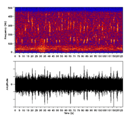
Tomographic transmissions consist of long coded signals (e.g., "m-sequences") lasting 30 seconds or more. The frequencies employed range from 50 to 1000 Hz and source powers range from 100 to 250 W, depending on the particular goals of the measurements. With precise timing such as from GPS, travel times can be measured to a nominal accuracy of 1 millisecond. While these transmissions are audible near the source, beyond a range of several kilometers the signals are usually below ambient noise levels, requiring sophisticated spread-spectrum signal processing techniques to recover them.
See also
- Underwater acoustics
- Acoustical oceanography
- Speed of sound
- SOFAR channel
- SOSUS
- Ray tracing
- TOPEX/Poseidon satellite altimetry
References
- 1 2 Munk, Walter; Peter Worcester; Carl Wunsch (1995). Ocean Acoustic Tomography. Cambridge: Cambridge University Press. ISBN 0-521-47095-1.
- ↑ Walter Sullivan (1987-07-28). "Vast Effort Aims to Reveal Oceans' Hidden Patterns". New York Times. Retrieved 2007-11-05.
- 1 2 "The Heard Island Feasibility Test". Acoustical Society of America. 1994.
- ↑ Munk, Walter; Carl Wunsch (1982). "Observing the ocean in the 1990s". Phil. Trans. R. Soc. Lond. A. 307 (1499): 439–464. Bibcode:1982RSPTA.307..439M. doi:10.1098/rsta.1982.0120.
- 1 2 Walter Munk (2006). History of Oceanography , M. Jochum and R. Murtugudde, eds., eds. Ocean Acoustic Tomography; from a stormy start to an uncertain future. New York: Springer.
- ↑ Fischer, A.S.; Hall, J.; Harrison, D.E.; Stammer, D.; Benveniste, J. (2010). "Conference Summary-Ocean Information for Society: Sustaining the Benefits, Realizing the Potential". In Hall, J.; Harrison, D.E.; Stammer, D. Proceedings of OceanObs’09: Sustained Ocean Observations and Information for Society (Vol. 1). ESA Publication WPP-306. Retrieved February 19, 2015.
- ↑ Pawlowicz, R.; et al. (1995-03-15). "Thermal evolution of the Greenland Sea gyre in 1988-1989". 100. Journal of Geophysical Research. pp. 4727–2750.
- ↑ Morawitz, W. M. L.; et al. (1996). "Three-dimensional observations of a deep convective chimney in the Greenland Sea during winter 1988/1989". 26. Journal of Physical Oceanography. pp. 2316–2343.
- ↑ Stammer, D.; et al. (2014). "Accuracy assessment of global barotropic ocean tide models". Reviews of Geophysics. 52: 243–282. Bibcode:2014RvGeo..52..243S. doi:10.1002/2014RG000450. Retrieved February 19, 2015.
- ↑ Dushaw, B.D.; Worcester, P.F.; Dzieciuch, M.A. (2011). "On the predictability of mode-1 internal tides". Deep-Sea Research Part I. 58: 677–698. Bibcode:2011DSRI...58..677D. doi:10.1016/j.dsr.2011.04.002. Retrieved February 19, 2015.
- ↑ Lebedev, K.V.; Yaremchuck, M.; Mitsudera, H.; Nakano, I.; Yuan, G. (2003). "Monitoring the Kuroshio Extension through dynamically constrained synthesis of the acoustic tomography, satellite altimeter and in situ data". Journal of Physical Oceanography. 59: 751–763. doi:10.1023/b:joce.0000009568.06949.c5.
- ↑ Mikhalevsky, P. N.; Gavrilov, A.N. (2001). "Acoustic thermometry in the Arctic Ocean". Polar Research. 20: 185–192. Bibcode:2001PolRe..20..185M. doi:10.1111/j.1751-8369.2001.tb00055.x. Retrieved February 19, 2015.
- ↑ Mikhalevsky, P. N.; Sagan, H.; et al. (2001). "Multipurpose acoustic networks in the integrated Arctic Ocean observing system". Arctic. 28, Suppl. 1: 17 pp. doi:10.14430/arctic4449. Retrieved April 24, 2015.
- ↑ Munk, W.H.; O'Reilly, W.C.; Reid, J.L. (1988). "Australia-Bermuda Sound Transmission Experiment (1960) Revisited.". Journal of Physical Oceanography. 18: 1876–1998. Bibcode:1988JPO....18.1876M. doi:10.1175/1520-0485(1988)018<1876:ABSTER>2.0.CO;2. Retrieved February 19, 2015.
- ↑ Dushaw, B.D.; Menemenlis, D. (2014). "Antipodal acoustic thermometry: 1960, 2004". Deep-Sea Research Part I. 86: 1–20. Bibcode:2014DSRI...86....1D. doi:10.1016/j.dsr.2013.12.008. Retrieved February 19, 2015.
- ↑ Spiesberger, john; Kurt Metzter (1992). "Basin scale ocean monitoring with acoustic thermometers". 5. Oceanography: 92–98.
- ↑ Spiesberger, J.L.; K. Metzger (1991). "Basin-scale tomography: A new tool for studying weather and climate". J. Geophys. Res. 96: 4869–4889. Bibcode:1991JGR....96.4869S. doi:10.1029/90JC02538.
- ↑ Spiesberger, John; Harley Hurlburt; Mark Johnson; Mark Keller; Steven Meyers; and J.J. O'Brien (1998). "Acoustic thermometry data compared with two ocean models: The importance of Rossby waves and ENSO in modifying the ocean interior". Dynamics of Atmospheres and Oceans. 26: 209–240. Bibcode:1998DyAtO..26..209S. doi:10.1016/s0377-0265(97)00044-4.
- ↑ The ATOC Consortium (1998-08-28). "Ocean Climate Change: Comparison of Acoustic Tomography, Satellite Altimetry, and Modeling". Science Magazine. pp. 1327–1332. Retrieved 2007-05-28.
- ↑ Dushaw, Brian; et al. (2009-07-19). "A decade of acoustic thermometry in the North Pacific Ocean". 114, C07021. J. Geophys. Res. doi:10.1029/2008JC005124.
- ↑ Stephanie Siegel (June 30, 1999). "Low-frequency sonar raises whale advocates' hackles". CNN. Retrieved 2007-10-23.
- ↑ Malcolm W. Browne (June 30, 1999). "Global Thermometer Imperiled by Dispute". NY Times. Retrieved 2007-10-23.
- ↑ Kenneth Chang (June 24, 1999). "An Ear to Ocean Temperature". ABC News. Archived from the original on 2003-10-06. Retrieved 2007-10-23.
- ↑ Potter, J. R. (1994). "ATOC: Sound Policy or Enviro-Vandalism? Aspects of a Modern Media-Fueled Policy Issue". 3. The Journal of Environment & Development. pp. 47–62. doi:10.1177/107049659400300205. Retrieved 2009-11-20.
- ↑ National Research Council (2000). Marine mammals and low-frequency sound: Progress since 1994. Washington, D.C.: National Academy Press.
- ↑ Frankel, A. S.; C. W. Clark (2000). "Behavioral responses of humpback whales (Megaptera novaeangliae) to full-scale ATOC signals". 108. Journal of the Acoustical Society of America. pp. 1–8. Retrieved 2009-08-15.
- ↑ Frankel, A. S.; C. W. Clark (2002). "ATOC and other factors affecting distribution and abundance of humpback whales (Megaptera novaeangliae) off the north shore of Kauai". 18. Marine Mammal Science. pp. 664–662. Retrieved 2009-08-15.
- ↑ Mobley, J. R. (2005). "Assessing responses of humpback whales to North Pacific Acoustic Laboratory (NPAL) transmissions: Results of 2001-2003 aerial surveys north of Kauai". 117. Journal of the Acoustical Society of America. pp. 1666–1673. Retrieved 2009-08-15.
- ↑ Bombosch, A. (2014). "Predictive habitat modelling of humpback (Megaptera novaeangliae) and Antarctic minke (Balaenoptera bonaerensis) whales in the Southern Ocean as a planning tool for seismic surveys". Deep-Sea Research Part I: Oceanographic Research Papers. Deep-Sea Research Part I. 91: 101–114. Bibcode:2014DSRI...91..101B. doi:10.1016/j.dsr.2014.05.017. Retrieved 2015-01-25.
- ↑ National Research Council (2003). Ocean Noise and Marine Mammals. National Academies Press. ISBN 978-0-309-08536-6. Retrieved 2015-01-25.
Further reading
- B. D. Dushaw, 2013. "Ocean Acoustic Tomography" in Encyclopedia of Remote Sensing, E. G. Njoku, Ed., Springer, Springer-Verlag Berlin Heidelberg, 2013. doi:10.1007/SpringerReference_331410
- W. Munk, P. Worcester, and C. Wunsch (1995). Ocean Acoustic Tomography. Cambridge: Cambridge University Press. ISBN 0-521-47095-1.
- P. F. Worcester, 2001: "Tomography," in Encyclopedia of Ocean Sciences, J. Steele, S. Thorpe, and K. Turekian, Eds., Academic Press Ltd., 2969–2986.
External links
- Oceans toolbox for Matlab by Rich Pawlowicz.
- Ocean Acoustics Lab (OAL) - the Woods Hole Oceanographic Institution.
- The North Pacific Acoustic Laboratory (NPAL) - the Scripps Institution of Oceanography, La Jolla, CA.
- Acoustic Thermometry of Ocean Climate - the Scripps Institution of Oceanography, La Jolla, CA.
- Discovery of Sound in the Sea - DOSITS is an educational website concerned with acoustics in the ocean.
- Sounds of acoustic signals employed for tomography - the DOSITS web page.
- A day in the life of a tomography mooring - University of Washington, Seattle, WA.
- Sounding Out the Ocean's Secrets - National Academy of Sciences.
- Sound Measures the Ocean's Secrets - Acoustical Society of America.
- The Acoustic Thermometry of Ocean Climate/Marine Mammal Research Program Cornell University Laboratory of Ornithology, Bioacoustics Research Program