Tomography

Fig.1: Basic principle of tomography: superposition free tomographic cross sections S₁ and S₂ compared with the projected image P

Fig.2: Optical coherence tomography of fingertip

Tomography refers to imaging by sections or sectioning, through the use of any kind of penetrating wave. The method is used in radiology, archaeology, biology, atmospheric science, geophysics, oceanography, plasma physics, materials science, astrophysics, quantum information, and other areas of science. In most cases the production of these images is based on the mathematical procedure tomographic reconstruction.

Overview

Tomography refers to imaging by sections or sectioning, through the use of any kind of penetrating wave or mechanical method. The method is used in radiology, archaeology, biology, atmospheric science, geophysics, oceanography, plasma physics, materials science, astrophysics, quantum information, and other sciences. In most cases it is based on the mathematical procedure called tomographic reconstruction.The word tomography is derived from Ancient Greek τόμος tomos, "slice, section" and γράφω graphō, "to write" (see also Etymology).

In conventional medical X-ray tomography, clinical staff make a sectional image through a body by moving an X-ray source and the film in opposite directions during the exposure. Consequently, structures in the focal plane appear sharper, while structures in other planes appear blurred.^[1] By modifying the direction and extent of the movement, operators can select different focal planes which contain the structures of interest. Before the advent of more modern computer-assisted techniques, this technique, developed in the 1930s by the radiologist Alessandro Vallebona, proved useful in reducing the problem of superimposition of structures in projectional (shadow) radiography.

Brief history

In a 1953 article in the medical journal Chest, B. Pollak of the Fort William Sanatorium described the use of planography, another term for tomography.^[2] A chapter in the American Roentgen Ray Society's 1996 book A History of the Radiological Sciences also provides a detailed history of the development of conventional tomography from its inception until being supplanted by computer assisted tomographic techniques starting in the mid to late-1970s.^[3]

A device used in tomography is called a tomograph, while the image produced is a tomogram. Tomography as the computed tomographic (CT) scanner was invented by Sir Godfrey Hounsfield, and thereby made an exceptional contribution to medicine.

Modern tomography

More modern variations of tomography involve gathering projection data from multiple directions and feeding the data into a tomographic reconstruction software algorithm processed by a computer.^[4] Different types of signal acquisition can be used in similar calculation algorithms in order to create a tomographic image. Tomograms are derived using several different physical phenomena listed in the following table:

Physical phenomenon	Type of tomogram
X-rays	CT
gamma rays	SPECT
radio-frequency waves	MRI
Electrical Resistance	ERT
Electrical Capacitance Tomography	ECT[5]
electron-positron annihilation	PET
electrons	Electron tomography or 3D TEM
muons	Muon tomography
ions	atom probe
magnetic particles	magnetic particle imaging
fluid flow	hydraulic tomography
Mid-infrared	Infrared microtomographic imaging[6]

Some recent advances rely on using simultaneously integrated physical phenomena, e.g. X-rays for both CT and angiography, combined CT/MRI and combined CT/PET.

The term volume imaging might describe these technologies more accurately than the term tomography. However, in the majority of cases in clinical routine, staff request output from these procedures as 2-D slice images. As more and more clinical decisions come to depend on more advanced volume visualization techniques, the terms tomography/tomogram may go out of fashion.

Many different reconstruction algorithms exist. Most algorithms fall into one of two categories: filtered back projection (FBP) and iterative reconstruction (IR). These procedures give inexact results: they represent a compromise between accuracy and computation time required. FBP demands fewer computational resources, while IR generally produces fewer artifacts (errors in the reconstruction) at a higher computing cost.^[4]

Although MRI and ultrasound are transmission methods, they typically do not require movement of the transmitter to acquire data from different directions. In MRI, both projections and higher spatial harmonics are sampled by applying spatially-varying magnetic fields; no moving parts are necessary to generate an image. On the other hand, since ultrasound uses time-of-flight to spatially encode the received signal, it is not strictly a tomographic method and does not require multiple acquisitions at all.

Basic principle

In this section, the basic principle of tomography in the case that especially uses tomography utilizing the parallel beam irradiation optical system will be explained.

Tomography is a technology that uses a tomographic optical system to obtain virtual 'slices' (a tomographic image) of specific cross section of a scanned object, allowing the user to see inside the object without cutting. There are several types of tomographic optical system including the parallel beam irradiation optical system. Parallel beam irradiation optical system may be the easiest and most practical example of a tomographic optical system therefore, in this article, explanation of "How to obtain the Tomographic image" will be based on "the parallel beam irradiation optical system". The resolution in tomography is typically described by the Crowther criterion.

Fig. 3: Considering a parallel beam irradiation optical system where the angle between the object and all transmission lights equals θ. Here, the numbers in the figure (see the numbers within the parentheses) respectively indicate: (1) = an object; (2) = the parallel beam light source; (3) = the screen; (4) = transmission beam; (5) = the datum circle; (6) = the origin; and (7) = a fluoroscopic image (a one-dimensional image; p_θ(s)). Two datum coordinate systems xy and ts are also imagined in order to explain the positional relations and movements of features (0)–(7) in the figure. In addition, a virtual circle centered at the above-mentioned origin (6) is set on the datum plane (it will be called “the datum circle” henceforth). This datum circle (6) represents the orbit of the parallel beam irradiation optical system. In the figure above, X-Y plane rotates around the point of origin in the plane in such a way “to keep mutual positional relationship between the light source (2) and screen (7) passing through the trajectory (5).” Rotation angle of this case is defined as θ. In the figure set out above, absorption coefficient at a cross-sectional coordinate (x, y) of the subject is modeled as μ(x, y).

The Fig. 3 is intended to illustrate the mathematical model and to illustrate the principle of tomography.In the Fig.3, absorption coefficient at a cross-sectional coordinate (x, y) of the subject is modeled as μ(x, y). Consideration based on the above assumptions may clarify the following items. Therefore, in this section, the explanation is advanced according to the order as follows:

• (1)Results of measurement, i.e. a series of images obtained by transmitted light are expressed (modeled) as a function p (s,θ) obtained by performing radon transform to μ(x, y), and
• (2)μ(x, y) is restored by performing inverse radon transform to measurement results.

(1)The Results of measurement p(s,θ) of parallel beam irradiation optical system

Considers the mathematical model such that the absorption coefficient of the object at each (x,y) are represented by μ(x,y) and one supposes that "the transmission beam penetrates without diffraction, diffusion, or reflection although it is absorbed by the object and its attenuation is assumed to occur in accordance with the Beer-Lambert law. In this matter, what we want to know” is μ(x,y) and what we can measure will be following p(s,θ).

When the attenuation is conformed to Beer-Lambert law, the relation between ${I}_{0}$ and $I$ is as following (eq.1) and therefore, the absorbance ($p_{l}$) along the light beam path (l(t)) is as following (eq.2). Here the ${I}_{0}$ is intensity of light beam before transmission $I$ is intensity of after transmission.

$I = I_0\exp\left({-\int\mu(x,y)\,dl}\right) = I_0\exp\left({-{\int}_{-\infty}^{\infty}\mu(l(t))\,|\dot{l}(t)|dt}\right)$ 　(eq. 1)

$p_{l} = \ln (I/I_0) = -\int\mu(x,y)\,dl = -{\int}_{-\infty}^{\infty}\mu(l(t))\,|\dot{l}(t)|dt$ (eq. 2)

Here, a direction from the light source toward the screen is defined as t direction and that perpendicular to t direction and parallel with the screen is defined as s direction. (Both t-s and x-y coordinate systems are set up such that they are reflected each other without mirror-reflective transformation.)

By using a parallel beam irradiation optical system, one can experimentally obtain the series of fluoroscopic images (a one-dimensional images” p_θ(s) of specific cross section of a scanned object) for each θ.　Here, θ　represents angle between the object and the transmission light beam. In the Fig.3, X-Y plane rotates counter clockwise ^{[Notes 1]} around the point of origin in the plane in such a way “to keep mutual positional relationship between the light source (2) and screen (7) passing through the trajectory (5).” Rotation angle of this case is same as above-mentioned θ.

The beam having an angle θ,to will be the collection of lays, represented by ${l}_{{[\theta ,s]}}(t)$ of following (eq. 3).

${l}_{{[\theta ,s]}}(t)=t{\begin{bmatrix}-\sin \theta \\\cos \theta \\\end{bmatrix}}+{\begin{bmatrix}s\cos \theta \\s\sin \theta \\\end{bmatrix}}$　(eq. 3)

The p_θ(s) is defined by following (eq. 4). That $p_{\theta}(s)$ is equal to the line integral of μ(x,y) along ${l}_{{[\theta ,s]}}(t)$ of (eq. 3) as the same manner of (eq.2). That means that, $p(s,\theta )$ of following (eq. 5) is a resultant of Radon transformation of μ(x,y).

$p_{{\theta }}(s)=-{\int }_{{-\infty }}^{{\infty }}\mu (s\cos \theta -t\sin \theta ,s\sin \theta +t\cos \theta )\,dt$　(eq. 4)

One can define following function of two variables (eq. 5). In this article, following p(s, θ) is called to be "the collection of fluoroscopic images".

p (s, θ)=p_θ(s)　　(eq. 5)

(2)μ(x, y) is restored by performing inverse radon transform to measurement results

“What we want to know (μ(x,y))” can be reconstructed from “What we majored ( p(s,θ))” by using inverse radon transformation . In the above-mentioned descriptions, “What we majored” is p(s,θ) . On the other hand, “What we want to know ” is μ(x,y). So, the next will be "How to reconstruct μ(x,y) from p(s,θ)".

Schematic configuration and motion

In this section, the schematic configuration and motion of the parallel beam irradiation optical system configured to obtain the p(s,θ) of above-mentioned (eq. 5) will be explained. In this section, how to obtain the p(s,θ) of (eq.5) by utilizing parallel beam irradiation optical system will also be explained. Configuration and motions of parallel beam irradiation optical system, referring the Fig. 3.

Statements

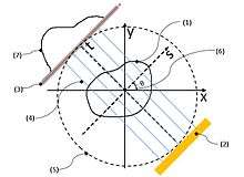
Numbers (1)–(7) shown in the Fig. 3 (see the numbers within the parentheses) respectively indicate: (1) = an object; (2) = the parallel beam light source; (3) = the screen; (4) = transmission beam; (5) = the datum circle (a datum feature); (6) = the origin (a datum feature); and (7) = a fluoroscopic image (a one-dimensional image; p (s, θ)).

Two datum coordinate systems xy and ts are imagined in order to explain the positional relations and movements of features (0)–(7) in the figure. The xy and ts coordinate systems share the origin (6) and they are positioned on the same plane. That is, the xy plane and the ts plane are the same plane. Henceforth, this virtual plane will be called “the datum plane”. In addition, a virtual circle centered at the abovementioned origin (6) is set on the datum plane (it will be called “the datum circle” henceforth). This datum circle (6) will be represents the orbit of the parallel beam irradiation optical system. Naturally, the origin (6), the datum circle (5), and the datum coordinate systems are virtual features which are imagined for mathematical purposes.

The μ(x,y) is absorption coefficient of the object (3) at each (x,y), p(s,θ) (7)is the collection of fluoroscopic images.

Motion of parallel beam irradiation optical system

The parallel beam irradiation optical system is the key component of a CT scanner. It consists of a parallel beam X-ray source (2) and the screen (3). They are positioned so that they face each other in parallel with the origin (6) in between, both being in contact with the datum circle (6).

These two features ((2) and (3)) can rotate counterclockwise ^{[Notes 1]} around the origin (6) together with the ts coordinate system while maintaining the relative positional relations between themselves and with the ts coordinate system (so, these two features ((2) and (3)) are always opposed each other). The ts plane is positioned so that the direction from a collimated X-ray source (2) to the screen (3) matches the positive direction of the t-axis while the s-axis parallels these two features. Henceforth, the angle between the x- and the s-axes will be indicated as θ. That is, parallel beam irradiation optical system where the angle between the object and the transmission beam equals θ. This datum circle (6) will be represents the orbit of the parallel beam irradiation optical system.

On the other hand, the object (1) will be scanned by CT scanner is fixed to xy coordination system. Hence, object (1) will not be moved while the parallel beam irradiation optical system are rotated around the object (1). The object (1) must be smaller than datum circle.

Obtaining transmission image ‘s’

During the above-mentioned motion (that is pivoting around the object(1)) of parallel beam irradiation optical system, the collimated X-ray source (2) emits transmission beam (4) which are effectively “parallel rays” in a geometrical optical sense. The traveling direction of each ray of the transmission beam (4) is parallel to the t-axis. The transmission beam (4), emitted by the X-ray source (2), penetrates the object and reaches the screen (3) after attenuation due to absorption by the object.

Optical transmission can be presumed to occur ideally. That is, transmission beam penetrates without diffraction, diffusion, or reflection although it is absorbed by the object and its attenuation is assumed to occur in accordance with the Beer-Lambert law.

Consequently, a fluoroscopic image (7) is recorded on the screen as a one-dimensional image (one image is recorded for every θ corresponding to all s values). When the angle between the object and transmission beam is θ and if the intensity of transmission beam (4) having reached each "s" point on the screen is expressed as p (s, θ), it expresses a fluoroscopic image (7) corresponding to each θ.

Types of tomography

Name	Source of data	Abbreviation	Year of introduction
Atom probe tomography	Atom probe	APT
Computed Tomography Imaging Spectrometer[7]	Visible light spectral imaging	CTIS
Confocal microscopy (Laser scanning confocal microscopy)	Laser scanning confocal microscopy	LSCM
Cryo-electron tomography	Cryo-electron microscopy	Cryo-ET
Electrical capacitance tomography	Electrical capacitance	ECT
Electrical resistivity tomography	Electrical resistivity	ERT
Electrical impedance tomography	Electrical impedance	EIT	1984
Electron tomography	Electron attenuation/scatter	ET
Functional magnetic resonance imaging	Magnetic resonance	fMRI	1992
Hydraulic tomography	fluid flow	HT	2000
Laser Ablation Tomography	Laser Ablation & Fluorescent Microscopy	LAT	2013
Magnetic induction tomography	Magnetic induction	MIT
Magnetic resonance imaging or nuclear magnetic resonance tomography	Nuclear magnetic moment	MRI or MRT
Muon tomography	muons
Microwave tomography[8]	Microwave (1-10 GHz electromagnetic radiation)
Neutron tomography	Neutron
Ocean acoustic tomography	Sonar
Optical coherence tomography	Interferometry	OCT
Optical diffusion tomography	Absorption of light	ODT
Optical projection tomography	Optical microscope	OPT
Photoacoustic imaging in biomedicine	Photoacoustic spectroscopy	PAT
Positron emission tomography	Positron emission	PET
Positron emission tomography - computed tomography	Positron emission & X-ray	PET-CT
Quantum tomography	Quantum state
Single photon emission computed tomography	Gamma ray	SPECT
Seismic tomography	Seismic waves
Terahertz tomography	Terahertz radiation	THz-CT
Thermoacoustic imaging	Photoacoustic spectroscopy	TAT
Ultrasound-modulated optical tomography	Ultrasound	UOT
Ultrasound computer tomography	Ultrasound	USCT
Ultrasound transmission tomography	Ultrasound
X-ray tomography	X-ray	CT, CATScan	1971
Zeeman-Doppler imaging	Zeeman effect

Discrete tomography and Geometric tomography, on the other hand, are research areas that deal with the reconstruction of objects that are discrete (such as crystals) or homogeneous. They are concerned with reconstruction methods, and as such they are not restricted to any of the particular (experimental) tomography methods listed above.

Synchrotron X-ray tomographic microscopy

A new technique called synchrotron X-ray tomographic microscopy (SRXTM) allows for detailed three-dimensional scanning of fossils.^[9]

The construction of third-generation synchrotron sources combined with the tremendous improvement of detector technology, data storage and processing capabilities since the 1990s has led to a boost of high-end synchrotron tomography in materials research with a wide range of different applications, e.g. the visualization and quantitative analysis of differently absorbing phases, microporosities, cracks, precipitates or grains in a specimen. Synchrotron radiation is created by accelerating free particles in high vacuum. By the laws of electrodynamics this acceleration leads to the emission of electromagnetic radiation (Jackson, 1975). Linear particle acceleration is one possibility, but apart from the very high electric fields one would need it is more practical to hold the charged particles on a closed trajectory in order to obtain a source of continuous radiation. Magnetic fields are used to force the particles onto the desired orbit and prevent them from flying in a straight line. The radial acceleration associated with the change of direction then generates radiation.^[10]

Use in Industry

Dredging & Mining

Industrial Tomography Systems (ITS)^[11] has collaborated with a leading European dredging contractor to develop their radiation and gamma free Dens-itometer.^[12] The system utilises electrical conductivity, to provide a greener, simpler, more cost effective alternative to conventional nuclear based systems.^[13] ITS pipe based sensors provide real time visual data on the processes occurring within the pipe.

The environmentally friendly Dens-itometer is making waves in the dredging and mining sector,^[14][15] as it can take measurements independent of flow regime and obtain readings of materials which are neutrally buoyant. The Dens-itometer has been tested on slurry conveying with 100,000s of tonnes of materials having been processed and delivering data consistent with gamma densitometers. It has also been deployed in food processing as a basis for measuring solids content in pipelines.^[12]

Mixing

Years of listening to industry professionals complain about their batch mixers has prompted Industrial Tomography Systems to develop the Mix-itometer,^[16] which utilises tomography solutions to resolve mixing problems. The Mix-itometer probe when placed inside batch mixers, replacing an existing baffle, measures average concentration and a mixing index by surveying more than 200 locations inside the process vessel.^[17] Mix-itometer software provides users with a visual representation of mixing upon a PC-based interface; the instrumentation produces real time volumetric imagery which gives producers a vividly detailed look of what occurs inside batch mixers.^[18]

See also

Media related to Tomography at Wikimedia Commons

• Chemical imaging
• Discrete tomography
• Geometric tomography
• Geophysical imaging
• Industrial CT scanning
• Medical imaging
• MRI compared with CT
• Network tomography
• Nonogram, a type of puzzle based on a discrete model of tomography
• Radon transform
• Tomographic reconstruction
• Multiscale Tomography
• Voxels

References

1. Tomography at the US National Library of Medicine Medical Subject Headings (MeSH)
2. Pollak, B. (December 1953). "Experiences with Planography". Chest. American College of Chest Physicians. 24 (6): 663–669. doi:10.1378/chest.24.6.663. ISSN 0012-3692. Retrieved July 10, 2011.
3. Littleton, J.T. "Conventional Tomography". A History of the Radiological Sciences (PDF). American Roentgen Ray Society. Retrieved 29 November 2014.
4. Herman, G. T., Fundamentals of computerized tomography: Image reconstruction from projection, 2nd edition, Springer, 2009
5. Industrial_Tomography_Systems
6. Martin; et al. (2013). "3D spectral imaging with synchrotron Fourier transform infrared spectro-microtomography". Nature Methods. 10: 861–864. doi:10.1038/nmeth.2596.
7. Ralf Habel, Michael Kudenov, Michael Wimmer: Practical Spectral Photography
8. Mojtaba Ahadi; et al. "Three dimensions localization of tumors in confocal microwave imaging for breast cancer detection". Microwave and Optical Technology Letters,Volume 57, Issue 12, pages 2917–2929, December 2015 . DOI: 10.1002/mop.29470
9. Donoghue; et al. (Aug 10, 2006). "Synchrotron X-ray tomographic microscopy of fossil embryos (letter)". Nature. 442 (7103): 680–683. Bibcode:2006Natur.442..680D. doi:10.1038/nature04890. PMID 16900198.
10. Banhart, John, ed. Advanced Tomographic Methods in Materials Research and Engineering. Monographs on the Physics and Chemistry of Materials. Oxford ; New York: Oxford University Press, 2008.
11. Industrial Tomography Systems, http://www.itoms.com/
12. Industrial Tomography Systems, http://www.itoms.com/products/gamma-densitometer-alternative/
13. Port Technnology, https://www.porttechnology.org/news/its_in_dredging_technology_master_plan
14. J. Butterworth, http://www.itoms.com/news/dens-itometer-steals-show-conference-brazil/
15. Dredge mag, http://www.dredgemag.com/September-October-2015/ITS-LAUNCHES-DENS-ITOMETER-FOR-SLURRY-MONITORING/
16. ITS, http://www.itoms.com/products/mixitometer/
17. ITS, http://www.itoms.com/wp-content/uploads/2013/01/ITS-MIX-ITOMETER-Brochure-online-version.pdf
18. laboratory Talk, http://laboratorytalk.com/article/2022181/mixing-up-personal-care

Notes

1. In this article, the following discussion is developed based on anticlockwise motion. But, whether the direction of the rotation is anti-clockwise or a clockwise is not an essential problem. Even if the rotational direction is assumed to be in an opposite direction, no specific impact is caused on essential level except for some minor deformation of formula including reversing a part of positive or negative signs.

External links

• Image reconstruction algorithms for microtomography