Generalized coordinates
| Classical mechanics |
|---|
|
Core topics |

In analytical mechanics, specifically the study of the rigid body dynamics of multibody systems, the term generalized coordinates refers to the parameters that describe the configuration of the system relative to some reference configuration. These parameters must uniquely define the configuration of the system relative to the reference configuration.[1] This is done assuming that this can be done with a single chart. The generalized velocities are the time derivatives of the generalized coordinates of the system.
An example of a generalized coordinate is the angle that locates a point moving on a circle. The adjective "generalized" distinguishes these parameters from the traditional use of the term coordinate to refer to Cartesian coordinates: for example, describing the location of the point on the circle using x and y coordinates.
Although there may be many choices for generalized coordinates for a physical system, parameters which are convenient are usually selected for the specification of the configuration of the system and which make the solution of its equations of motion easier. If these parameters are independent of one another, the number of independent generalized coordinates is defined by the number of degrees of freedom of the system.[2][3]
Constraints and degrees of freedom
Generalized coordinates are usually selected to provide the minimum number of independent coordinates that define the configuration of a system, which simplifies the formulation of Lagrange's equations of motion. However, it can also occur that a useful set of generalized coordinates may be dependent, which means that they are related by one or more constraint equations.
Holonomic constraints
For a system of N particles in 3D real coordinate space, the position vector of each particle can be written as a 3-tuple in Cartesian coordinates:

Any of the position vectors can be denoted rk where k = 1, 2, ..., N labels the particles. A holonomic constraint is a constraint equation of the form for particle k[4][nb 1]

which connects all the 3 spatial coordinates of that particle together, so they are not independent. The constraint may change with time, so time t will appear explicitly in the constraint equations. At any instant of time, when t is a constant, any one coordinate will be determined from the other coordinates, e.g. if xk and zk are given, then so is yk. One constraint equation counts as one constraint. If there are C constraints, each has an equation, so there will be C constraint equations. There is not necessarily one constraint equation for each particle, and if there are no constraints on the system then there are no constraint equations.
So far, the configuration of the system is defined by 3N quantities, but C coordinates can be eliminated, one coordinate from each constraint equation. The number of independent coordinates is n = 3N − C. (In D dimensions, the original configuration would need ND coordinates, and the reduction by constraints means n = ND − C). It is ideal to use the minimum number of coordinates needed to define the configuration of the entire system, while taking advantage of the constraints on the system. These quantities are known as generalized coordinates in this context, denoted qj(t). It is convenient to collect them into an n-tuple

which is a point in the configuration space of the system. They are all independent of one other, and each is a function of time. Geometrically they can be lengths along straight lines, or arc lengths along curves, or angles; not necessarily Cartesian coordinates or other standard orthogonal coordinates. There is one for each degree of freedom, so the number of generalized coordinates equals the number of degrees of freedom, n. A degree of freedom corresponds to one quantity that changes the configuration of the system, for example the angle of a pendulum, or the arc length traversed by a bead along a wire.
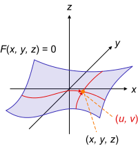
If it is possible to find from the constraints as many independent variables as there are degrees of freedom, these can be used as generalized coordinates[5] The position vector rk of particle k is a function of all the n generalized coordinates and time,[6][7][8][5][nb 2]

and the generalized coordinates can be thought of as parameters associated with the constraint.
The corresponding time derivatives of q are the generalized velocities,

(each dot over a quantity indicates one time derivative). The velocity vector vk is the total derivative of rk with respect to time

and so generally depends on the generalized velocities and coordinates. Since we are free to specify the initial values of the generalized coordinates and velocities separately, the generalized coordinates and velocities can be treated as independent variables. The generalized coordinates qj and velocities dqj/dt are treated as independent variables.
Non-holonomic constraints
A mechanical system can involve constraints on both the generalized coordinates and their derivatives. Constraints of this type are known as non-holonomic. First-order non-holonomic constraints have the form

An example of such a constraint is a rolling wheel or knife-edge that constrains the direction of the velocity vector. Non-holonomic constraints can also involve next-order derivatives such as generalized accelerations.
Physical quantities in generalized coordinates
Kinetic energy
The total kinetic energy of the system is the energy of the system's motion, defined as[9]

in which · is the dot product. The kinetic energy is a function only of the velocities vk, not the coordinates rk themselves. By contrast an important observation is[10]

which illustrates the kinetic energy is in general a function of the generalized velocities, coordinates, and time if the constraint also varies with time, so T = T(q, dq/dt, t).
In the case the constraint on the particle is time-independent, then all partial derivatives with respect to time are zero, and the kinetic energy has no time-dependence and is a homogeneous function of degree 2 in the generalized velocities;

Still for the time-independent case, this expression is equivalent to taking the line element squared of the trajectory for particle k,

and dividing by the square differential in time, dt2, to obtain the velocity squared of particle k. Thus for time-independent constraints it is sufficient to know the line element to quickly obtain the kinetic energy of particles and hence the Lagrangian.[11]
It is instructive to see the various cases of polar coordinates in 2d and 3d, owing to their frequent appearance. In 2d polar coordinates (r, θ),

in 3d cylindrical coordinates (r, θ, z),

in 3d spherical coordinates (r, θ, φ),

Generalized momentum
The generalized momentum "canonically conjugate to" the coordinate qi is defined by

If the Lagrangian L does not depend on some coordinate qi, then it follows from the Euler–Lagrange equations that the corresponding generalized momentum will be a conserved quantity, because the time derivative is zero implying the momentum is a constant of the motion;

Examples
Bead on a wire
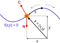
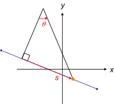
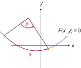
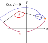
For a bead sliding on a frictionless wire subject only to gravity in 2d space, the constraint on the bead can be stated in the form f(r) = 0, where the position of the bead can be written r = (x(s), y(s)), in which s is a parameter, the arc length s along the curve from some point on the wire. This is a suitable choice of generalized coordinate for the system. Only one coordinate is needed instead of two, because the position of the bead can be parameterized by one number, s, and the constraint equation connects the two coordinates x and y; either one is determined from the other. The constraint force is the reaction force the wire exerts on the bead to keep it on the wire, and the non-constraint applied force is gravity acting on the bead.
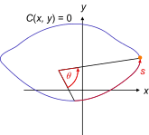
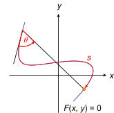
Suppose the wire changes its shape with time, by flexing. Then the constraint equation and position of the particle are respectively

which now both depend on time t due to the changing coordinates as the wire changes its shape. Notice time appears implicitly via the coordinates and explicitly in the constraint equations.
Simple pendulum
The relationship between the use of generalized coordinates and Cartesian coordinates to characterize the movement of a mechanical system can be illustrated by considering the constrained dynamics of a simple pendulum.[12][13]
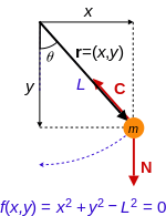
A simple pendulum consists of a mass M hanging from a pivot point so that it is constrained to move on a circle of radius L. The position of the mass is defined by the coordinate vector r=(x, y) measured in the plane of the circle such that y is in the vertical direction. The coordinates x and y are related by the equation of the circle

that constrains the movement of M. This equation also provides a constraint on the velocity components,

Now introduce the parameter θ, that defines the angular position of M from the vertical direction. It can be used to define the coordinates x and y, such that

The use of θ to define the configuration of this system avoids the constraint provided by the equation of the circle.
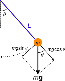
Notice that the force of gravity acting on the mass m is formulated in the usual Cartesian coordinates,

where g is the acceleration of gravity.
The virtual work of gravity on the mass m as it follows the trajectory r is given by

The variation δr can be computed in terms of the coordinates x and y, or in terms of the parameter θ,

Thus, the virtual work is given by

Notice that the coefficient of δy is the y-component of the applied force. In the same way, the coefficient of δθ is known as the generalized force along generalized coordinate θ, given by

To complete the analysis consider the kinetic energy T of the mass, using the velocity,

so,

D'Alembert's form of the principle of virtual work for the pendulum in terms of the coordinates x and y are given by,

This yields the three equations

in the three unknowns, x, y and λ.
Using the parameter θ, those equations take the form

which becomes,

or

This formulation yields one equation because there is a single parameter and no constraint equation.
This shows that the parameter θ is a generalized coordinate that can be used in the same way as the Cartesian coordinates x and y to analyze the pendulum.
Double pendulum
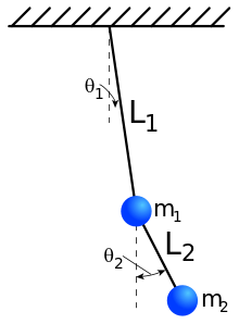
The benefits of generalized coordinates become apparent with the analysis of a double pendulum. For the two masses mi, i=1, 2, let ri=(xi, yi), i=1, 2 define their two trajectories. These vectors satisfy the two constraint equations,

The formulation of Lagrange's equations for this system yields six equations in the four Cartesian coordinates xi, yi i=1, 2 and the two Lagrange multipliers λi, i=1, 2 that arise from the two constraint equations.
Now introduce the generalized coordinates θi i=1,2 that define the angular position of each mass of the double pendulum from the vertical direction. In this case, we have

The force of gravity acting on the masses is given by,

where g is the acceleration of gravity. Therefore, the virtual work of gravity on the two masses as they follow the trajectories ri, i=1,2 is given by

The variations δri i=1, 2 can be computed to be

Thus, the virtual work is given by

and the generalized forces are

Compute the kinetic energy of this system to be

Euler–Lagrange equation yield two equations in the unknown generalized coordinates θi i=1, 2, given by[14]

and

The use of the generalized coordinates θi i=1, 2 provides an alternative to the Cartesian formulation of the dynamics of the double pendulum.
Spherical pendulum
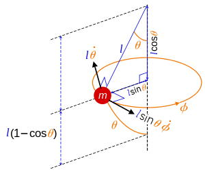
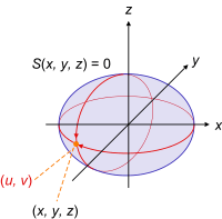
For a 3d example, a spherical pendulum with constant length l free to swing in any angular direction subject to gravity, the constraint on the pendulum bob can be stated in the form

where the position of the pendulum bob can be written

in which (θ, φ) are the spherical polar angles because the bob moves in the surface of a sphere. The position r is measured along the suspension point to the bob, here treated as a point particle. A logical choice of generalized coordinates to describe the motion are the angles (θ, φ). Only two coordinates are needed instead of three, because the position of the bob can be parameterized by two numbers, and the constraint equation connects the three coordinates x, y, z so any one of them is determined from the other two.
Generalized coordinates and virtual work
The principle of virtual work states that if a system is in static equilibrium, the virtual work of the applied forces is zero for all virtual movements of the system from this state, that is, δW=0 for any variation δr.[15] When formulated in terms of generalized coordinates, this is equivalent to the requirement that the generalized forces for any virtual displacement are zero, that is Fi=0.
Let the forces on the system be Fj, j=1, ..., m be applied to points with Cartesian coordinates rj, j=1,..., m, then the virtual work generated by a virtual displacement from the equilibrium position is given by

where δrj, j=1, ..., m denote the virtual displacements of each point in the body.
Now assume that each δrj depends on the generalized coordinates qi, i=1, ..., n, then

and

The n terms

are the generalized forces acting on the system. Kane[16] shows that these generalized forces can also be formulated in terms of the ratio of time derivatives,

where vj is the velocity of the point of application of the force Fj.
In order for the virtual work to be zero for an arbitrary virtual displacement, each of the generalized forces must be zero, that is

See also
- Hamiltonian mechanics
- Virtual work
- Orthogonal coordinates
- Curvilinear coordinates
- Mass matrix
- Stiffness matrix
- Generalized forces
Notes
- ↑ Some authors set the constraint equations to a constant for convenience with some constraint equations (e.g. pendulums), others set it to zero. It makes no difference because the constant can be subtracted to give zero on one side of the equation. Also, in Lagrange's equations of the first kind, only the derivatives are needed.
- ↑ Some authors e.g. Hand & Finch take the form of the position vector for particle k, as shown here, as the condition for the constraint on that particle to be holonomic.
References
- ↑ Ginsberg 2008, p. 397, §7.2.1 Selection of generalized coordinates
- ↑ Farid M. L. Amirouche (2006). "§2.4: Generalized coordinates". Fundamentals of multibody dynamics: theory and applications. Springer. p. 46. ISBN 0-8176-4236-6.
- ↑ Florian Scheck (2010). "§5.1 Manifolds of generalized coordinates". Mechanics: From Newton's Laws to Deterministic Chaos (5th ed.). Springer. p. 286. ISBN 3-642-05369-6.
- ↑ Goldstein 1980, p. 12
- 1 2 Kibble & Berkshire 2004, p. 232
- ↑ Torby 1984, p. 260
- ↑ Goldstein 1980, p. 13
- ↑ Hand & Finch 2008, p. 15
- ↑ Torby 1984, p. 269
- ↑ Goldstein 1980, p. 25
- ↑ Landau & Lifshitz 1976, p. 8
- ↑ Greenwood, Donald T. (1987). Principles of Dynamics (2nd ed.). Prentice Hall. ISBN 0-13-709981-9.
- ↑ Richard Fitzpatrick, Newtonian Dynamics, http://farside.ph.utexas.edu/teaching/336k/Newton/Newtonhtml.html.
- ↑ Eric W. Weisstein, Double Pendulum, scienceworld.wolfram.com. 2007
- ↑ Torby, Bruce (1984). "Energy Methods". Advanced Dynamics for Engineers. HRW Series in Mechanical Engineering. United States of America: CBS College Publishing. ISBN 0-03-063366-4.
- ↑ T. R. Kane and D. A. Levinson, Dynamics: theory and applications, McGraw-Hill, New York, 1985
Bibliography of cited references
- Ginsberg, Jerry H. (2008). Engineering dynamics (3rd ed.). Cambridge UK: Cambridge University Press. ISBN 978-0-521-88303-0.
- Kibble, T.W.B; Berkshire, F.H. (2004). Classical Mechanics (5th ed.). River Edge NJ: Imperial College Press. ISBN 1860944248.