Gauss–Newton algorithm
The Gauss–Newton algorithm is used to solve non-linear least squares problems. It is a modification of Newton's method for finding a minimum of a function. Unlike Newton's method, the Gauss–Newton algorithm can only be used to minimize a sum of squared function values, but it has the advantage that second derivatives, which can be challenging to compute, are not required.
Non-linear least squares problems arise for instance in non-linear regression, where parameters in a model are sought such that the model is in good agreement with available observations.
The method is named after the mathematicians Carl Friedrich Gauss and Isaac Newton.
Description
Given m functions r = (r1, …, rm) (often called residuals) of n variables β = (β1, …, βn), with m ≥ n, the Gauss–Newton algorithm iteratively finds the value of the variables which minimizes the sum of squares[1]

Starting with an initial guess for the minimum, the method proceeds by the iterations


where, if r and β are column vectors, the entries of the Jacobian matrix are

and the symbol denotes the matrix transpose.

If m = n, the iteration simplifies to

which is a direct generalization of Newton's method in one dimension.
In data fitting, where the goal is to find the parameters β such that a given model function y = f(x, β) best fits some data points (xi, yi), the functions ri are the residuals

Then, the Gauss-Newton method can be expressed in terms of the Jacobian Jf of the function f as

Notes
The assumption m ≥ n in the algorithm statement is necessary, as otherwise the matrix JrTJr is not invertible and the normal equations cannot be solved (at least uniquely).
The Gauss–Newton algorithm can be derived by linearly approximating the vector of functions ri. Using Taylor's theorem, we can write at every iteration:

with The task of finding Δ minimizing the sum of squares of the right-hand side, i.e.,

- ,

is a linear least squares problem, which can be solved explicitly, yielding the normal equations in the algorithm.
The normal equations are m linear simultaneous equations in the unknown increments, Δ. They may be solved in one step, using Cholesky decomposition, or, better, the QR factorization of Jr. For large systems, an iterative method, such as the conjugate gradient method, may be more efficient. If there is a linear dependence between columns of Jr, the iterations will fail as JrTJr becomes singular.
Example


In this example, the Gauss–Newton algorithm will be used to fit a model to some data by minimizing the sum of squares of errors between the data and model's predictions.
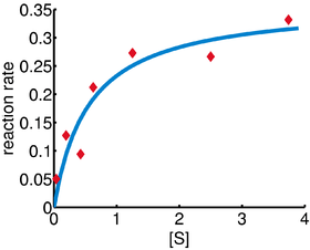
In a biology experiment studying the relation between substrate concentration [S] and reaction rate in an enzyme-mediated reaction, the data in the following table were obtained.
i 1 2 3 4 5 6 7 [S] 0.038 0.194 0.425 0.626 1.253 2.500 3.740 rate 0.050 0.127 0.094 0.2122 0.2729 0.2665 0.3317
It is desired to find a curve (model function) of the form
![\text{rate}=\frac{V_\text{max}[S]}{K_M+[S]}](../I/m/634484edf21bcda03f43725ed42aebcd19ce5311.svg)
that fits best the data in the least squares sense, with the parameters and to be determined.


Denote by and the value of [S] and the rate from the table, Let and We will find and such that the sum of squares of the residuals


is minimized.
The Jacobian of the vector of residuals in respect to the unknowns is an matrix with the -th row having the entries


Starting with the initial estimates of and , after five iterations of the Gauss–Newton algorithm the optimal values and are obtained. The sum of squares of residuals decreased from the initial value of 1.445 to 0.00784 after the fifth iteration. The plot in the figure on the right shows the curve determined by the model for the optimal parameters versus the observed data.


Convergence properties
It can be shown[2] that the increment Δ is a descent direction for S, and, if the algorithm converges, then the limit is a stationary point of S. However, convergence is not guaranteed, not even local convergence as in Newton's method, or convergence under the usual Wolfe conditions .[3]
The rate of convergence of the Gauss–Newton algorithm can approach quadratic.[4] The algorithm may converge slowly or not at all if the initial guess is far from the minimum or the matrix is ill-conditioned. For example, consider the problem with equations and variable, given by


The optimum is at . (Actually the optimum is at for , because , but .) If then the problem is in fact linear and the method finds the optimum in one iteration. If |λ| < 1 then the method converges linearly and the error decreases asymptotically with a factor |λ| at every iteration. However, if |λ| > 1, then the method does not even converge locally.[5]


Derivation from Newton's method
In what follows, the Gauss–Newton algorithm will be derived from Newton's method for function optimization via an approximation. As a consequence, the rate of convergence of the Gauss–Newton algorithm can be quadratic under certain regularity conditions. In general (under weaker conditions), the convergence rate is linear.[6]
The recurrence relation for Newton's method for minimizing a function S of parameters, , is


where g denotes the gradient vector of S and H denotes the Hessian matrix of S. Since , the gradient is given by


Elements of the Hessian are calculated by differentiating the gradient elements, , with respect to


The Gauss–Newton method is obtained by ignoring the second-order derivative terms (the second term in this expression). That is, the Hessian is approximated by

where are entries of the Jacobian Jr. The gradient and the approximate Hessian can be written in matrix notation as


These expressions are substituted into the recurrence relation above to obtain the operational equations

Convergence of the Gauss–Newton method is not guaranteed in all instances. The approximation

that needs to hold to be able to ignore the second-order derivative terms may be valid in two cases, for which convergence is to be expected.[7]
- The function values are small in magnitude, at least around the minimum.
- The functions are only "mildly" non linear, so that is relatively small in magnitude.

Improved versions
With the Gauss–Newton method the sum of squares of the residuals S may not decrease at every iteration. However, since Δ is a descent direction, unless is a stationary point, it holds that for all sufficiently small . Thus, if divergence occurs, one solution is to employ a fraction, , of the increment vector, Δ in the updating formula:


- .

In other words, the increment vector is too long, but it points in "downhill", so going just a part of the way will decrease the objective function S. An optimal value for can be found by using a line search algorithm, that is, the magnitude of is determined by finding the value that minimizes S, usually using a direct search method in the interval .

In cases where the direction of the shift vector is such that the optimal fraction, , is close to zero, an alternative method for handling divergence is the use of the Levenberg–Marquardt algorithm, also known as the "trust region method".[1] The normal equations are modified in such a way that the increment vector is rotated towards the direction of steepest descent,
- ,

where D is a positive diagonal matrix. Note that when D is the identity matrix I and , then , therefore the direction of Δ approaches the direction of the negative gradient .


The so-called Marquardt parameter, , may also be optimized by a line search, but this is inefficient as the shift vector must be re-calculated every time is changed. A more efficient strategy is this. When divergence occurs increase the Marquardt parameter until there is a decrease in S. Then, retain the value from one iteration to the next, but decrease it if possible until a cut-off value is reached when the Marquardt parameter can be set to zero; the minimization of S then becomes a standard Gauss–Newton minimization.

Large-scale optimization
For large scale optimization, the Gauss-Newton method is of special interest because it is often (though certainly not always) true that the matrix is more sparse than the approximate Hessian . In such cases, the step calculation itself will typically need to be done with an approximate iterative method appropriate for large and sparse problems, such as the conjugate gradient method.


In order to make this kind of approach work, one needs at minimum an efficient method for computing the product

for some vector p. With sparse matrix storage, it is in general practical to store the rows of in a compressed form (eg, without zero entries), making a direct computation of the above product tricky due to the transposition. However, if one defines ci as row i of the matrix , the following simple relation holds

so that every row contributes additively and independently to the product. In addition to respecting a practical sparse storage structure, this expression is well suited for parallel computations. Note that every row ci is the gradient of the corresponding residual ri; with this in mind, the formula above emphasizes the fact that residuals contribute to the problem independently of each other.
Related algorithms
In a quasi-Newton method, such as that due to Davidon, Fletcher and Powell or Broyden–Fletcher–Goldfarb–Shanno (BFGS method) an estimate of the full Hessian, , is built up numerically using first derivatives only so that after n refinement cycles the method closely approximates to Newton's method in performance. Note that quasi-Newton methods can minimize general real-valued functions, whereas Gauss-Newton, Levenberg-Marquardt, etc. fits only to nonlinear least-squares problems.


Another method for solving minimization problems using only first derivatives is gradient descent. However, this method does not take into account the second derivatives even approximately. Consequently, it is highly inefficient for many functions, especially if the parameters have strong interactions.
Notes
- 1 2 Björck (1996)
- ↑ Björck (1996) p260
- ↑ Mascarenhas (2013), "The divergence of the BFGS and Gauss Newton Methods", Mathematical Programming, 147 (1): 253–276, doi:10.1007/s10107-013-0720-6
- ↑ Björck (1996) p341, 342
- ↑ Fletcher (1987) p.113
- ↑ http://www.henley.ac.uk/web/FILES/maths/09-04.pdf
- ↑ Nocedal (1999) p259
References
- Björck, A. (1996). Numerical methods for least squares problems. SIAM, Philadelphia. ISBN 0-89871-360-9.
- Fletcher, Roger (1987). Practical methods of optimization (2nd ed.). New York: John Wiley & Sons. ISBN 978-0-471-91547-8..
- Nocedal, Jorge; Wright, Stephen (1999). Numerical optimization. New York: Springer. ISBN 0-387-98793-2.
External links
Implementations
- Artelys Knitro is a non-linear solver with an implementation of the Gauss-Newton method. It is written in C and has interfaces to C++/C#/Java/Python/MATLAB/R.
|  | |||||||||||||||||||||||||||
|
| ||||||||||||||||||||||||||||
| ||||||||||||||||||||||||||||
| ||||||||||||||||||||||||||||