Variance
In probability theory and statistics, variance is the expectation of the squared deviation of a random variable from its mean, and it informally measures how far a set of (random) numbers are spread out from their mean. The variance has a central role in statistics. It is used in descriptive statistics, statistical inference, hypothesis testing, goodness of fit, Monte Carlo sampling, amongst many others. This makes it a central quantity in numerous fields such as physics, biology, chemistry, economics, and finance. The variance is the square of the standard deviation, the second central moment of a distribution, and the covariance of the random variable with itself, and it is often represented by , , or .


Definition
The variance of a random variable is the expected value of the squared deviation from the mean of , :

![{\displaystyle \mu =\operatorname {E} [X]}](../I/m/ce1b41598b8e8f45f57c1550ebb8d5c7ab8e1210.svg)
![\operatorname {Var} (X)=\operatorname {E} \left[(X-\mu )^{2}\right].](../I/m/55622d2a1cf5e46f2926ab389a8e3438edb53731.svg)
This definition encompasses random variables that are generated by processes that are discrete, continuous, neither, or mixed. The variance can also be thought of as the covariance of a random variable with itself:

The variance is also equivalent to the second cumulant of a probability distribution that generates . The variance is typically designated as , , or simply (pronounced "sigma squared"). The expression for the variance can be expanded:

![{\begin{aligned}\operatorname {Var} (X)&=\operatorname {E} \left[(X-\operatorname {E} [X])^{2}\right]\\&=\operatorname {E} \left[X^{2}-2X\operatorname {E} [X]+(\operatorname {E} [X])^{2}\right]\\&=\operatorname {E} \left[X^{2}\right]-2\operatorname {E} [X]\operatorname {E} [X]+(\operatorname {E} [X])^{2}\\&=\operatorname {E} \left[X^{2}\right]-(\operatorname {E} [X])^{2}\end{aligned}}](../I/m/86060a001d3617ca85ed73efb63ec7908d77fa5f.svg)
A mnemonic for the above expression is "mean of square minus square of mean". On computational floating point arithmetic, this equation should not be used, because it suffers from catastrophic cancellation if the two components of the equation are similar in magnitude. There exist numerically stable alternatives.
Continuous random variable
If the random variable represents samples generated by a continuous distribution with probability density function , then the population variance is given by


where is the expected value


and where the integrals are definite integrals taken for ranging over the range of .

If a continuous distribution does not have an expected value, as is the case for the Cauchy distribution, it does not have a variance either. Many other distributions for which the expected value does exist also do not have a finite variance because the integral in the variance definition diverges. An example is a Pareto distribution whose index satisfies .


Discrete random variable
If the generator of random variable is discrete with probability mass function then


or equivalently

where is the expected value, i.e.

(When such a discrete weighted variance is specified by weights whose sum is not 1, then one divides by the sum of the weights.)
The variance of a set of equally likely values can be written as


where is the expected value, i.e.,

The variance of a set of equally likely values can be equivalently expressed, without directly referring to the mean, in terms of squared deviations of all points from each other:[1]

Examples
Normal distribution
The normal distribution with parameters and is a continuous distribution whose probability density function is given by


In this distribution, and the variance is related with via
![{\displaystyle \operatorname {E} [X]=\mu }](../I/m/9e19f2ee2d8e606b7b96a6667b3e8cd403851b53.svg)

The role of the normal distribution in the central limit theorem is in part responsible for the prevalence of the variance in probability and statistics.
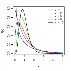
Exponential distribution
The exponential distribution with parameter is a continuous distribution whose support is the semi-infinite interval . Its probability density function is given by

![{\displaystyle \left[0,\infty \right]}](../I/m/6b2116a6b40568aabe1eaf29b9677503552cb976.svg)

and it has expected value . The variance is equal to


So for an exponentially distributed random variable, .

Poisson distribution
The Poisson distribution with parameter is a discrete distribution for . Its probability mass function is given by


and it has expected value . The variance is equal to


So for a Poisson-distributed random variable, .

Binomial distribution
The binomial distribution with parameters and is a discrete distribution for . Its probability mass function is given by


and it has expected value . The variance is equal to


Coin toss
The binomial distribution with describes the probability of getting heads in tosses. Thus the expected value of the number of heads is , and the variance is .


Fair die
A six-sided fair die can be modelled with a discrete random variable with outcomes 1 through 6, each with equal probability . The expected value is . Therefore, the variance can be computed to be


The general formula for the variance of the outcome X of a die of n sides is

Properties
Basic properties
Variance is non-negative because the squares are positive or zero.

The variance of a constant random variable is zero, and if the variance of a variable in a data set is 0, then all the entries have the same value.

Variance is invariant with respect to changes in a location parameter. That is, if a constant is added to all values of the variable, the variance is unchanged.

If all values are scaled by a constant, the variance is scaled by the square of that constant.

The variance of a sum of two random variables is given by:


where Cov(⋅, ⋅) is the covariance. In general we have for the sum of random variables :


These results lead to the variance of a linear combination as:

If the random variables are such that


they are said to be uncorrelated. It follows immediately from the expression given earlier that if the random variables are uncorrelated, then the variance of their sum is equal to the sum of their variances, or, expressed symbolically:

Since independent random variables are always uncorrelated, the equation above holds in particular when the random variables are independent. Thus independence is sufficient but not necessary for the variance of the sum to equal the sum of the variances.

Sum of uncorrelated variables (Bienaymé formula)
One reason for the use of the variance in preference to other measures of dispersion is that the variance of the sum (or the difference) of uncorrelated random variables is the sum of their variances:

This statement is called the Bienaymé formula[2] and was discovered in 1853. It is often made with the stronger condition that the variables are independent, but being uncorrelated suffices. So if all the variables have the same variance σ2, then, since division by n is a linear transformation, this formula immediately implies that the variance of their mean is

That is, the variance of the mean decreases when n increases. This formula for the variance of the mean is used in the definition of the standard error of the sample mean, which is used in the central limit theorem.
Sum of correlated variables
In general, if the variables are correlated, then the variance of their sum is the sum of their covariances:

(Note: The second equality comes from the fact that Cov(Xi,Xi) = Var(Xi).)
Here Cov(⋅, ⋅) is the covariance, which is zero for independent random variables (if it exists). The formula states that the variance of a sum is equal to the sum of all elements in the covariance matrix of the components. This formula is used in the theory of Cronbach's alpha in classical test theory.
So if the variables have equal variance σ2 and the average correlation of distinct variables is ρ, then the variance of their mean is

This implies that the variance of the mean increases with the average of the correlations. In other words, additional correlated observations are not as effective as additional independent observations at reducing the uncertainty of the mean. Moreover, if the variables have unit variance, for example if they are standardized, then this simplifies to

This formula is used in the Spearman–Brown prediction formula of classical test theory. This converges to ρ if n goes to infinity, provided that the average correlation remains constant or converges too. So for the variance of the mean of standardized variables with equal correlations or converging average correlation we have

Therefore, the variance of the mean of a large number of standardized variables is approximately equal to their average correlation. This makes clear that the sample mean of correlated variables does not generally converge to the population mean, even though the Law of large numbers states that the sample mean will converge for independent variables.
Matrix notation for the variance of a linear combination
Define as a column vector of random variables , and as a column vector of scalars . Therefore, is a linear combination of these random variables, where denotes the transpose of . Also let be the covariance matrix of . The variance of is then given by:[3]


Weighted sum of variables
The scaling property and the Bienaymé formula, along with the property of the covariance Cov(aX, bY) = ab Cov(X, Y) jointly imply that

This implies that in a weighted sum of variables, the variable with the largest weight will have a disproportionally large weight in the variance of the total. For example, if X and Y are uncorrelated and the weight of X is two times the weight of Y, then the weight of the variance of X will be four times the weight of the variance of Y.
The expression above can be extended to a weighted sum of multiple variables:

Product of independent variables
If two variables X and Y are independent, the variance of their product is given by[4]
![{\begin{aligned}\operatorname {Var} (XY)&=[E(X)]^{2}\operatorname {Var} (Y)+[E(Y)]^{2}\operatorname {Var} (X)+\operatorname {Var} (X)\operatorname {Var} (Y).\end{aligned}}](../I/m/78ba93b03d6960ae5d2a0bd47d027cd2354c9d36.svg)
Equivalently, using the basic properties of expectation, it is given by
![\operatorname {Var} (XY)=E(X^{2})E(Y^{2})-[E(X)]^{2}[E(Y)]^{2}.](../I/m/e431a2d861b74d8df6334564e9cdf79be994a6f8.svg)
Product of correlated variables
In general, if two variables are correlated, the variance of their product is given by:
![{\begin{aligned}\operatorname {Var} (XY)&=E[X^{2}Y^{2}]-[E(XY)]^{2}\\&=\operatorname {Cov} (X^{2},Y^{2})+E(X^{2})E(Y^{2})-[E(XY)]^{2}\\&=\operatorname {Cov} (X^{2},Y^{2})+(\operatorname {Var} (X)+[E(X)]^{2})(\operatorname {Var} (Y)+[E(Y)]^{2})-[\operatorname {Cov} (X,Y)+E(X)E(Y)]^{2}\end{aligned}}](../I/m/f69eebf38df8850d0a28086083d2791a159b0875.svg)
Decomposition
The general formula for variance decomposition or the law of total variance is: If and are two random variables, and the variance of exists, then

![\operatorname {Var} [X]=\operatorname {E} _{Y}(\operatorname {Var} [X\mid Y])+\operatorname {Var} _{Y}(\operatorname {E} [X\mid Y]).\,](../I/m/e7773e42d6187e16a7b15671d92064282394cfce.svg)
where is the conditional expectation of given , and is the conditional variance of given . (A more intuitive explanation is that given a particular value of , then follows a distribution with mean and variance ). As is a function of the variable , the outer expectation or variance is taken with respect to Y. The above formula tells how to find based on the distributions of these two quantities when is allowed to vary.


In particular, if is a discrete random variable assuming with corresponding probability masses , then in the formula for total variance, the first term on the right-hand side becomes


![{\displaystyle \operatorname {E} _{Y}(\operatorname {Var} [X\mid Y])=\sum _{i=1}^{n}p_{i}\sigma _{i}^{2},}](../I/m/8e19d6962933e6675cdecedcd41ef9af549d77fa.svg)
where . Similarly, the second term on the right-hand side becomes
![{\displaystyle \sigma _{i}^{2}=\operatorname {Var} [X\mid y_{i}]}](../I/m/e8be4fd216f532a9b361e210bed15515915a7150.svg)
![{\displaystyle \operatorname {Var} _{Y}(\operatorname {E} [X\mid Y])=\sum _{i=1}^{n}p_{i}\mu _{i}^{2}-\left(\sum _{i=1}^{n}p_{i}\mu _{i}\right)^{2}=\sum _{i=1}^{n}p_{i}\mu _{i}^{2}-\mu ^{2},}](../I/m/67f7c447b64128dca8a745fd8daf0966ee2af82f.svg)
where and . Thus the total variance is given by
![{\displaystyle \mu _{i}=\operatorname {E} [X\mid y_{i}]}](../I/m/cdccc3d3570982fdcd1851e5f87fdc99d74df173.svg)

![{\displaystyle \operatorname {Var} [X]=\sum _{i=1}^{n}p_{i}\sigma _{i}^{2}+\left(\sum _{i=1}^{n}p_{i}\mu _{i}^{2}-\mu ^{2}\right).}](../I/m/80bd24748644e9be42a70be6ffe8f01691f7587e.svg)
A similar formula is applied in analysis of variance, where the corresponding formula is

here refers to the Mean of the Squares. In linear regression analysis the corresponding formula is


This can also be derived from the additivity of variances, since the total (observed) score is the sum of the predicted score and the error score, where the latter two are uncorrelated.
Similar decompositions are possible for the sum of squared deviations (sum of squares, ):


Formulae for the variance
A formula often used for deriving the variance of a theoretical distribution is as follows:

This will be useful when it is possible to derive formulae for the expected value and for the expected value of the square.
This formula is also sometimes used in connection with the sample variance. While useful for hand calculations, it is not advised for computer calculations as it suffers from catastrophic cancellation if the two components of the equation are similar in magnitude and floating point arithmetic is used. This is discussed in the article Algorithms for calculating variance.
Calculation from the CDF
The population variance for a non-negative random variable can be expressed in terms of the cumulative distribution function F using

This expression can be used to calculate the variance in situations where the CDF, but not the density, can be conveniently expressed.
Characteristic property
The second moment of a random variable attains the minimum value when taken around the first moment (i.e., mean) of the random variable, i.e. . Conversely, if a continuous function satisfies for all random variables X, then it is necessarily of the form , where a > 0. This also holds in the multidimensional case.[5]


Units of measurement
Unlike expected absolute deviation, the variance of a variable has units that are the square of the units of the variable itself. For example, a variable measured in meters will have a variance measured in meters squared. For this reason, describing data sets via their standard deviation or root mean square deviation is often preferred over using the variance. In the dice example the standard deviation is √2.9 ≈ 1.7, slightly larger than the expected absolute deviation of 1.5.
The standard deviation and the expected absolute deviation can both be used as an indicator of the "spread" of a distribution. The standard deviation is more amenable to algebraic manipulation than the expected absolute deviation, and, together with variance and its generalization covariance, is used frequently in theoretical statistics; however the expected absolute deviation tends to be more robust as it is less sensitive to outliers arising from measurement anomalies or an unduly heavy-tailed distribution.
Approximating the variance of a function
The delta method uses second-order Taylor expansions to approximate the variance of a function of one or more random variables: see Taylor expansions for the moments of functions of random variables. For example, the approximate variance of a function of one variable is given by
![\operatorname {Var} \left[f(X)\right]\approx \left(f'(\operatorname {E} \left[X\right])\right)^{2}\operatorname {Var} \left[X\right]](../I/m/8c58412ffa8fdf818b89bafb3318c4ace7cd8e9b.svg)
provided that f is twice differentiable and that the mean and variance of X are finite.
Population variance and sample variance
Real-world observations such as the measurements of yesterday's rain throughout the day typically cannot be complete sets of all possible observations that could be made. As such, the variance calculated from the finite set will in general not match the variance that would have been calculated from the full population of possible observations. This means that one estimates the mean and variance that would have been calculated from an omniscient set of observations by using an estimator equation. The estimator is a function of the sample of n observations drawn without observational bias from the whole population of potential observations. In this example that sample would be the set of actual measurements of yesterday's rainfall from available rain gauges within the geography of interest.
The simplest estimators for population mean and population variance are simply the mean and variance of the sample, the sample mean and (uncorrected) sample variance – these are consistent estimators (they converge to the correct value as the number of samples increases), but can be improved. Estimating the population variance by taking the sample's variance is close to optimal in general, but can be improved in two ways. Most simply, the sample variance is computed as an average of squared deviations about the (sample) mean, by dividing by n. However, using values other than n improves the estimator in various ways. Four common values for the denominator are n, n − 1, n + 1, and n − 1.5: n is the simplest (population variance of the sample), n − 1 eliminates bias, n + 1 minimizes mean squared error for the normal distribution, and n − 1.5 mostly eliminates bias in unbiased estimation of standard deviation for the normal distribution.
Firstly, if the omniscient mean is unknown (and is computed as the sample mean), then the sample variance is a biased estimator: it underestimates the variance by a factor of (n − 1) / n; correcting by this factor (dividing by n − 1 instead of n) is called Bessel's correction. The resulting estimator is unbiased, and is called the (corrected) sample variance or unbiased sample variance. For example, when n = 1 the variance of a single observation about the sample mean (itself) is obviously zero regardless of the population variance. If the mean is determined in some other way than from the same samples used to estimate the variance then this bias does not arise and the variance can safely be estimated as that of the samples about the (independently known) mean.
Secondly, the sample variance does not generally minimize mean squared error between sample variance and population variance. Correcting for bias often makes this worse: one can always choose a scale factor that performs better than the corrected sample variance, though the optimal scale factor depends on the excess kurtosis of the population (see mean squared error: variance), and introduces bias. This always consists of scaling down the unbiased estimator (dividing by a number larger than n − 1), and is a simple example of a shrinkage estimator: one "shrinks" the unbiased estimator towards zero. For the normal distribution, dividing by n + 1 (instead of n − 1 or n) minimizes mean squared error. The resulting estimator is biased, however, and is known as the biased sample variation.
Population variance
In general, the population variance of a finite population of size N with values xi is given by

where the population mean is
- .

The population variance can also be computed using

This is true because

The population variance matches the variance of the generating probability distribution. In this sense, the concept of population can be extended to continuous random variables with infinite populations.
Sample variance
In many practical situations, the true variance of a population is not known a priori and must be computed somehow. When dealing with extremely large populations, it is not possible to count every object in the population, so the computation must be performed on a sample of the population.[6] Sample variance can also be applied to the estimation of the variance of a continuous distribution from a sample of that distribution.
We take a sample with replacement of n values y1, ..., yn from the population, where n < N, and estimate the variance on the basis of this sample.[7] Directly taking the variance of the sample data gives the average of the squared deviations:

Here, denotes the sample mean:


Since the yi are selected randomly, both and are random variables. Their expected values can be evaluated by summing over the ensemble of all possible samples {yi} from the population. For this gives:


![{\begin{aligned}E[\sigma _{y}^{2}]&=E\left[{\frac {1}{n}}\sum _{i=1}^{n}\left(y_{i}-{\frac {1}{n}}\sum _{j=1}^{n}y_{j}\right)^{2}\right]\\&={\frac {1}{n}}\sum _{i=1}^{n}E\left[y_{i}^{2}-{\frac {2}{n}}y_{i}\sum _{j=1}^{n}y_{j}+{\frac {1}{n^{2}}}\sum _{j=1}^{n}y_{j}\sum _{k=1}^{n}y_{k}\right]\\&={\frac {1}{n}}\sum _{i=1}^{n}\left[{\frac {n-2}{n}}E[y_{i}^{2}]-{\frac {2}{n}}\sum _{j\neq i}E[y_{i}y_{j}]+{\frac {1}{n^{2}}}\sum _{j=1}^{n}\sum _{k\neq j}^{n}E[y_{j}y_{k}]+{\frac {1}{n^{2}}}\sum _{j=1}^{n}E[y_{j}^{2}]\right]\\&={\frac {1}{n}}\sum _{i=1}^{n}\left[{\frac {n-2}{n}}(\sigma ^{2}+\mu ^{2})-{\frac {2}{n}}(n-1)\mu ^{2}+{\frac {1}{n^{2}}}n(n-1)\mu ^{2}+{\frac {1}{n}}(\sigma ^{2}+\mu ^{2})\right]\\&={\frac {n-1}{n}}\sigma ^{2}.\end{aligned}}](../I/m/174ff8a2df764acb89eda2fc2c0588f846226dce.svg)
Hence gives an estimate of the population variance that is biased by a factor of . For this reason, is referred to as the biased sample variance. Correcting for this bias yields the unbiased sample variance:


Either estimator may be simply referred to as the sample variance when the version can be determined by context. The same proof is also applicable for samples taken from a continuous probability distribution.
The use of the term n − 1 is called Bessel's correction, and it is also used in sample covariance and the sample standard deviation (the square root of variance). The square root is a concave function and thus introduces negative bias (by Jensen's inequality), which depends on the distribution, and thus the corrected sample standard deviation (using Bessel's correction) is biased. The unbiased estimation of standard deviation is a technically involved problem, though for the normal distribution using the term n − 1.5 yields an almost unbiased estimator.
The unbiased sample variance is a U-statistic for the function ƒ(y1, y2) = (y1 − y2)2/2, meaning that it is obtained by averaging a 2-sample statistic over 2-element subsets of the population.
Distribution of the sample variance

Being a function of random variables, the sample variance is itself a random variable, and it is natural to study its distribution. In the case that yi are independent observations from a normal distribution, Cochran's theorem shows that s2 follows a scaled chi-squared distribution:[8]

As a direct consequence, it follows that

and[9]
![\operatorname {Var} [s^{2}]=\operatorname {Var} \left({\frac {\sigma ^{2}}{n-1}}\chi _{n-1}^{2}\right)={\frac {\sigma ^{4}}{(n-1)^{2}}}\operatorname {Var} \left(\chi _{n-1}^{2}\right)={\frac {2\sigma ^{4}}{n-1}}.](../I/m/d1240e22b54bede05c0d8ab0c9a0479a5583e222.svg)
If the yi are independent and identically distributed, but not necessarily normally distributed, then[10][11]
![\operatorname {E} [s^{2}]=\sigma ^{2},\quad \operatorname {Var} [s^{2}]={\frac {\sigma ^{4}}{n}}\left((\kappa -1)+{\frac {2}{n-1}}\right)={\frac {1}{n}}\left(\mu _{4}-{\frac {n-3}{n-1}}\sigma ^{4}\right),](../I/m/836f92da5719c874e2f8c61bc0bf2ece4c8fb7ea.svg)
where κ is the kurtosis of the distribution and μ4 is the fourth central moment.
If the conditions of the law of large numbers hold for the squared observations, s2 is a consistent estimator of σ2. One can see indeed that the variance of the estimator tends asymptotically to zero. An asymptotically equivalent formula was given in Kenney and Keeping (1951:164), Rose and Smith (2002:264), and Weisstein (n.d.).[12][13][14]
Samuelson's inequality
Samuelson's inequality is a result that states bounds on the values that individual observations in a sample can take, given that the sample mean and (biased) variance have been calculated.[15] Values must lie within the limits

Relations with the harmonic and arithmetic means
It has been shown[16] that for a sample {yi} of real numbers,

where ymax is the maximum of the sample, A is the arithmetic mean, H is the harmonic mean of the sample and is the (biased) variance of the sample.

This bound has been improved, and it is known that variance is bounded by


where ymin is the minimum of the sample.[17]
Tests of equality of variances
Testing for the equality of two or more variances is difficult. The F test and chi square tests are both adversely affected by non-normality and are not recommended for this purpose.
Several non parametric tests have been proposed: these include the Barton–David–Ansari–Freund–Siegel–Tukey test, the Capon test, Mood test, the Klotz test and the Sukhatme test. The Sukhatme test applies to two variances and requires that both medians be known and equal to zero. The Mood, Klotz, Capon and Barton–David–Ansari–Freund–Siegel–Tukey tests also apply to two variances. They allow the median to be unknown but do require that the two medians are equal.
The Lehmann test is a parametric test of two variances. Of this test there are several variants known. Other tests of the equality of variances include the Box test, the Box–Anderson test and the Moses test.
Resampling methods, which include the bootstrap and the jackknife, may be used to test the equality of variances.
History
The term variance was first introduced by Ronald Fisher in his 1918 paper The Correlation Between Relatives on the Supposition of Mendelian Inheritance:[18]
The great body of available statistics show us that the deviations of a human measurement from its mean follow very closely the Normal Law of Errors, and, therefore, that the variability may be uniformly measured by the standard deviation corresponding to the square root of the mean square error. When there are two independent causes of variability capable of producing in an otherwise uniform population distributions with standard deviations and , it is found that the distribution, when both causes act together, has a standard deviation . It is therefore desirable in analysing the causes of variability to deal with the square of the standard deviation as the measure of variability. We shall term this quantity the Variance...


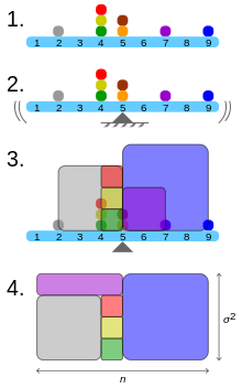
- A frequency distribution is constructed.
- The centroid of the distribution gives its mean.
- A square with sides equal to the difference of each value from the mean is formed for each value.
- Arranging the squares into a rectangle with one side equal to the number of values, n, results in the other side being the distribution's variance, σ².
Moment of inertia
The variance of a probability distribution is analogous to the moment of inertia in classical mechanics of a corresponding mass distribution along a line, with respect to rotation about its center of mass. It is because of this analogy that such things as the variance are called moments of probability distributions. The covariance matrix is related to the moment of inertia tensor for multivariate distributions. The moment of inertia of a cloud of n points with a covariance matrix of is given by

This difference between moment of inertia in physics and in statistics is clear for points that are gathered along a line. Suppose many points are close to the x axis and distributed along it. The covariance matrix might look like

That is, there is the most variance in the x direction. Physicists would consider this to have a low moment about the x axis so the moment-of-inertia tensor is

Semivariance
The semivariance is calculated in the same manner as the variance but only those observations that fall below the mean are included in the calculation. It is sometimes described as a measure of downside risk in an investments context. For skewed distributions, the semivariance can provide additional information that a variance does not.
Generalizations
If is a scalar complex-valued random variable, with values in , then its variance is , where is the complex conjugate of . This variance is a real scalar.


If is a vector-valued random variable, with values in , and thought of as a column vector, then the natural generalization of variance is , where and is the transpose of , and so is a row vector. The result is a positive semi-definite square matrix, commonly referred to as the variance-covariance matrix.


If is a vector- and complex-valued random variable, with values in , then the generalization of its variance is , where is the conjugate transpose of . This matrix is also positive semi-definite and square.


See also
| Look up variance in Wiktionary, the free dictionary. |
- Algorithms for calculating variance
- Average absolute deviation
- Bhatia–Davis inequality
- Common-method variance
- Correlation
- Covariance
- Chebyshev's inequality
- Distance variance
- Estimation of covariance matrices
- Explained variance
- Homoscedasticity
- Mean absolute error
- Mean absolute difference
- Mean preserving spread
- Pooled variance (also known as combined, composite, or overall variance)
- Popoviciu's inequality on variances
- Qualitative variation
- Sample mean and covariance
- Reduced chi-squared
- Semivariance
- Skewness
- Taylor's law
- Weighted sample variance
Notes
- ↑ Yuli Zhang,Huaiyu Wu,Lei Cheng (June 2012). Some new deformation formulas about variance and covariance. Proceedings of 4th International Conference on Modelling, Identification and Control(ICMIC2012). pp. 987–992.
- ↑ Loeve, M. (1977) "Probability Theory", Graduate Texts in Mathematics, Volume 45, 4th edition, Springer-Verlag, p. 12.
- ↑ Johnson, Richard; Wichern, Dean (2001). Applied Multivariate Statistical Analysis. Prentice Hall. p. 76. ISBN 0-13-187715-1
- ↑ Goodman, Leo A., "On the exact variance of products," Journal of the American Statistical Association, December 1960, 708–713. DOI: 10.2307/2281592
- ↑ Kagan, A.; Shepp, L. A. (1998). "Why the variance?". Statistics & Probability Letters. 38 (4): 329–333. doi:10.1016/S0167-7152(98)00041-8.
- ↑ Navidi, William (2006) Statistics for Engineers and Scientists, McGraw-Hill, pg 14.
- ↑ Montgomery, D. C. and Runger, G. C. (1994) Applied statistics and probability for engineers, page 201. John Wiley & Sons New York
- ↑ Knight K. (2000), Mathematical Statistics, Chapman and Hall, New York. (proposition 2.11)
- ↑ Casella and Berger (2002) Statistical Inference, Example 7.3.3, p. 331
- ↑ Cho, Eungchun; Cho, Moon Jung; Eltinge, John (2005) The Variance of Sample Variance From a Finite Population. International Journal of Pure and Applied Mathematics 21 (3): 387-394. http://www.ijpam.eu/contents/2005-21-3/10/10.pdf
- ↑ Cho, Eungchun; Cho, Moon Jung (2009) Variance of Sample Variance With Replacement. International Journal of Pure and Applied Mathematics 52 (1): 43-47. http://www.ijpam.eu/contents/2009-52-1/5/5.pdf
- ↑ Kenney, John F.; Keeping, E.S. (1951) Mathematics of Statistics. Part Two. 2nd ed. D. Van Nostrand Company, Inc. Princeton: New Jersey. http://krishikosh.egranth.ac.in/bitstream/1/2025521/1/G2257.pdf
- ↑ Rose, Colin; Smith, Murray D. (2002) Mathematical Statistics with Mathematica. Springer-Verlag, New York. http://www.mathstatica.com/book/Mathematical_Statistics_with_Mathematica.pdf
- ↑ Weisstein, Eric W. (n.d.) Sample Variance Distribution. MathWorld--A Wolfram Web Resource. http://mathworld.wolfram.com/SampleVarianceDistribution.html
- ↑ Samuelson, Paul (1968). "How Deviant Can You Be?". Journal of the American Statistical Association. 63 (324): 1522–1525. doi:10.1080/01621459.1968.10480944. JSTOR 2285901.
- ↑ Mercer, A. McD. (2000). "Bounds for A–G, A–H, G–H, and a family of inequalities of Ky Fan's type, using a general method". J. Math. Anal. Appl. 243 (1): 163–173. doi:10.1006/jmaa.1999.6688.
- ↑ Sharma, R. (2008). "Some more inequalities for arithmetic mean, harmonic mean and variance". J. Math. Inequalities. 2 (1): 109–114. doi:10.7153/jmi-02-11.
- ↑ Ronald Fisher (1918) The correlation between relatives on the supposition of Mendelian Inheritance
Theory of probability distributions | ||
|---|---|---|
 | ||
| |||||||||||||||||||||||||||||||||||||||||||||
| |||||||||||||||||||||||||||||||||||||||||||||
| |||||||||||||||||||||||||||||||||||||||||||||
| |||||||||||||||||||||||||||||||||||||||||||||
| |||||||||||||||||||||||||||||||||||||||||||||
| |||||||||||||||||||||||||||||||||||||||||||||
| |||||||||||||||||||||||||||||||||||||||||||||