Standard error
The standard error (SE) is the standard deviation of the sampling distribution of a statistic,[1] most commonly of the mean.
The standard error of the mean (SEM) can be seen to depict the relationship between the dispersion of individual observations around the population mean (the standard deviation), and the dispersion of sample means around the population mean (the standard error). Different samples drawn from that same population would in general have different values of the sample mean, so there is a distribution of sampled means (with its own mean and variance). The relationship with the standard deviation is defined such that, for a given sample size, the standard error equals the standard deviation divided by the square root of the sample size. As the sample size increases, the dispersion of the sample means clusters more closely around the population mean and the standard error decreases.
In regression analysis, the term "standard error" is also used in the phrase standard error of the regression to mean the ordinary least squares estimate of the standard deviation of the underlying errors.[2][3] The term may also be used to refer to an estimate of that standard deviation, derived from a particular sample used to compute the estimate.
Introduction to the standard error
The standard error is a quantitative measure of uncertainty. Consider the following scenarios.
Scenario 1. For an upcoming national election, 2000 voters are chosen at random and asked if they will vote for candidate A or candidate B. Of the 2000 voters, 1040 (52%) state that they will vote for candidate A. The researchers report that candidate A is expected to receive 52% of the final vote, with a margin of error of 2%. In this scenario, the 2000 voters are a sample from all the actual voters. The sample proportion of 52% is an estimate of the true proportion who will vote for candidate A in the actual election. The margin of error of 2% is a quantitative measure of the uncertainty – the possible difference between the true proportion who will vote for candidate A and the estimate of 52%.
Scenario 2. A medical research team tests a new drug to lower cholesterol. They report that, in a sample of 400 patients, the new drug lowers cholesterol by an average of 20 units (mg/dL). The 95% confidence interval for the average effect of the drug is that it lowers cholesterol by 18 to 22 units. In this scenario, the 400 patients are a sample of all patients who may be treated with the drug. The confidence interval of 18 to 22 is a quantitative measure of the uncertainty – the possible difference between the true average effect of the drug and the estimate of 20 mg/dL.
In each of these scenarios, a sample of observations is drawn from a large population. The proportion or the mean is calculated using the sample. Because of random variation in sampling, the proportion or mean calculated using the sample will usually differ from the true proportion or mean in the entire population. A quantitative measure of uncertainty is reported: a margin of error of 2%, or a confidence interval of 18 to 22. The margin of error and the confidence interval are based on a quantitative measure of uncertainty: the standard error. The standard error of a proportion and the standard error of the mean describe the possible variability of the estimated value based on the sample around the true proportion or true mean
Standard errors are used in many hypothesis tests, such as t-tests. They may be used to calculate confidence intervals.
Standard error of the mean (SEM)
This section will focus on the standard error of the mean. Later sections will present the standard error of other statistics, such as the standard error of a proportion, the standard error of the difference of two means, the standard error of the difference of two proportions and so on.
The concept of a sampling distribution is key to understanding the standard error. Two data sets will be helpful to illustrate the concept of a sampling distribution and its use to calculate the standard error. As will be shown, the standard error is the standard deviation of the sampling distribution.
Sampling from a distribution with a large standard deviation
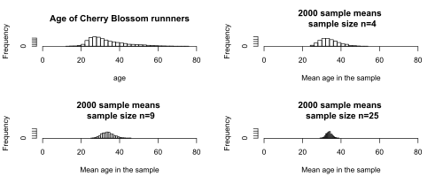
The first data set consists of the ages of 9,732 women who completed the 2012 Cherry Blossom run, a 10-mile race held in Washington each spring. The age data are in the data set run10 from the R package openintro that accompanies the textbook by Dietz [4]
The graph shows the distribution of ages for the runners.
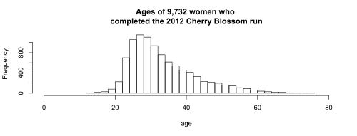
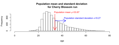
For the purpose of this example, the 9,732 runners who completed the 2012 run are the entire population of interest. The mean age was 33.88 years. The standard deviation of the age was 9.27 years. Because the 9,732 runners are the entire population, 33.88 years is the population mean, , and 9.27 years is the population standard deviation, σ. Greek letters indicate that these are population values.

Consider a sample of n=16 runners selected at random from the 9,732. The ages in one such sample are 23, 27, 28, 29, 31, 31, 32, 33, 34, 38, 40, 40, 48, 53, 54, and 55. The graph shows the ages for the 16 runners in the sample, plotted on the distribution of ages for all 9,732 runners.
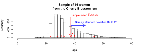
The mean age for the 16 runners in this particular sample is 37.25. The standard deviation of the age for the 16 runners is 10.23. Because these 16 runners are a sample from the population of 9,732 runners, 37.25 is the sample mean, and 10.23 is the sample standard deviation, s. Roman letters indicate that these are sample values. The sample mean = 37.25 is greater than the true population mean = 33.88 years. The sample standard deviation s = 10.23 is greater than the true population standard deviation σ = 9.27 years. For any random sample from a population, the sample mean will very rarely be equal to the population mean. Similarly, the sample standard deviation will very rarely be equal to the population standard deviation.

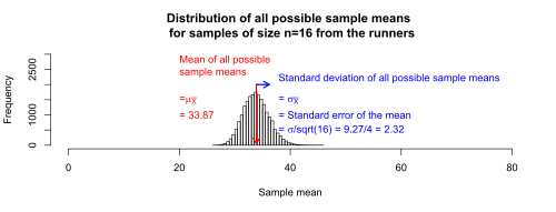
Next, consider all possible samples of 16 runners from the population of 9,732 runners. For each sample, the mean age of the 16 runners in the sample can be calculated. The distribution of the mean age in all possible samples is called the sampling distribution of the mean. For illustration, the graph below shows the distribution of the sample means for 20,000 samples, where each sample is of size n=16.
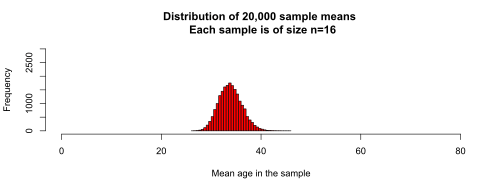
The next graph shows the sampling distribution of the mean (the distribution of the 20,000 sample means) superimposed on the distribution of ages for the 9,732 women.
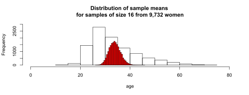
The distribution of these 20,000 sample means indicate how far the mean of a sample may be from the true population mean. A natural way to describe the variation of these sample means around the true population mean is the standard deviation of the distribution of the sample means.

The mean of all possible sample means is equal to the population mean. For the runners, the population mean age is 33.87, and the population standard deviation is 9.27. It will be shown that the standard deviation of all possible sample means of size n=16 is equal to the population standard deviation, σ, divided by the square root of the sample size, 16. This gives 9.27/sqrt(16) = 2.32. The standard deviation of all possible sample means is the standard error, and is represented by the symbol .

Sampling from a distribution with a small standard deviation
The second data set consists of the age at first marriage of 5,534 US women who responded to the National Survey of Family Growth (NSFG) conducted by the CDC in the 2006 and 2010 cycle. The data set is ageAtMar, also from the R package openintro from the textbook by Dietz et al.[4]
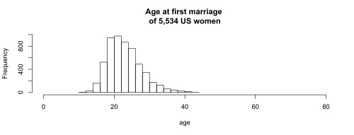
For the purpose of this example, the 5,534 women are the entire population of interest. The mean age was 23.44 years. The standard deviation of the age was 4.72 years. Because the 5,534 women are the entire population, 23.44 years is the population mean, , and 4.72 years is the population standard deviation, .

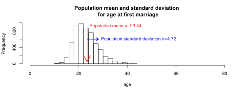
Notice that the population standard deviation of 4.72 years for age at first marriage is about half the standard deviation of 9.27 years for the runners. The smaller standard deviation for age at first marriage will result in a smaller standard error of the mean.
Repeating the sampling procedure as for the Cherry Blossom runners, take 20,000 samples of size n=16 from the age at first marriage population. The graph below shows the distribution of the sample means for 20,000 samples, where each sample is of size n=16.
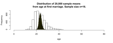
The mean of these 20,000 samples from the age at first marriage population is 23.44, and the standard deviation of the 20,000 sample means is 1.18.
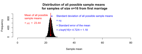
As will be shown, the mean of all possible sample means is equal to the population mean. For the age at first marriage, the population mean age is 23.44, and the population standard deviation is 4.72. It will be shown that the standard deviation of all possible sample means of size n=16 is equal to the population standard deviation, σ, divided by the square root of the sample size, 16, which is 4.72/sqrt(16) = 1.18. The standard deviation of all possible sample means of size 16 is the standard error.
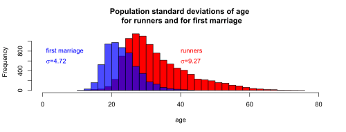
It is useful to compare the standard error of the mean for the age of the runners versus the age at first marriage, as in the graph.
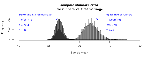
Because the age of the runners have a larger standard deviation (9.27 years) than does the age at first marriage (4.72 years), the standard error of the mean is larger for the runners than for first marriage.
Larger sample sizes give smaller standard errors
As would be expected, larger sample sizes give smaller standard errors. The graphs below show the sampling distribution of the mean for samples of size 4, 9, and 25. As the sample size increases, the sampling distribution become more narrow, and the standard error decreases.
Using a sample to estimate the standard error
In the examples so far, the population standard deviation σ was assumed to be known. If σ is known, the standard error is calculated using the formula

where
- σ is the standard deviation of the population.
- n is the size (number of observations) of the sample.
It is rare that the true population standard deviation is known. However, the sample standard deviation, s, is an estimate of σ. If σ is not known, the standard error is estimated using the formula

where
- s is the sample standard deviation
- n is the size (number of observations) of the sample.
Notice that is only an estimate of the true standard error, .
In an example above, n=16 runners were selected at random from the 9,732 runners. The ages in that sample were 23, 27, 28, 29, 31, 31, 32, 33, 34, 38, 40, 40, 48, 53, 54, and 55. The standard deviation of the age for the 16 runners is 10.23, which is somewhat greater than the true population standard deviation σ = 9.27 years. Compare the true standard error of the mean to the standard error estimated using this sample.
The true standard error of the mean, using σ = 9.27, is

The standard error of the mean estimated by using the sample standard deviation, s = 10.23, is

The true standard error of the mean is 2.32. The standard error estimated using the sample standard deviation is 2.56.
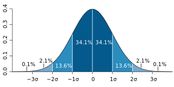
For the purpose of hypothesis testing or estimating confidence intervals, the standard error is primarily of use when the sampling distribution is normally distributed, or approximately normally distributed. These assumptions may be approximately met when the population from which samples are taken is normally distributed, or when the sample size is sufficiently large to rely on the Central Limit Theorem.
Standard error of the mean
The standard error of the mean (SEM) is the standard deviation of the sample-mean's estimate of a population mean. (It can also be viewed as the standard deviation of the error in the sample mean with respect to the true mean, since the sample mean is an unbiased estimator.) SEM is usually estimated by the sample estimate of the population standard deviation (sample standard deviation) divided by the square root of the sample size (assuming statistical independence of the values in the sample):

where
- s is the sample standard deviation (i.e., the sample-based estimate of the standard deviation of the population), and
- n is the size (number of observations) of the sample.
This estimate may be compared with the formula for the true standard deviation of the sample mean:

where
- σ is the standard deviation of the population.
This formula may be derived from what we know about the variance of a sum of independent random variables.[5]
- If are independent observations from a population that has a mean and standard deviation , then the variance of the total is
- The variance of must be
- And the standard deviation of must be .
- Of course, is the sample mean .


Note: the standard error and the standard deviation of small samples tend to systematically underestimate the population standard error and deviations: the standard error of the mean is a biased estimator of the population standard error. With n = 2 the underestimate is about 25%, but for n = 6 the underestimate is only 5%. Gurland and Tripathi (1971)[6] provide a correction and equation for this effect. Sokal and Rohlf (1981)[7] give an equation of the correction factor for small samples of n < 20. See unbiased estimation of standard deviation for further discussion.
A practical result: Decreasing the uncertainty in a mean value estimate by a factor of two requires acquiring four times as many observations in the sample. Or decreasing standard error by a factor of ten requires a hundred times as many observations.
Student approximation when σ value is unknown
In many practical applications, the true value of σ is unknown. As a result, we need to use a distribution that takes into account that spread of possible σ's. When the true underlying distribution is known to be Gaussian, although with unknown σ, then the resulting estimated distribution follows the Student t-distribution. The standard error is the standard deviation of the Student t-distribution. T-distributions are slightly different from Gaussian, and vary depending on the size of the sample. To estimate the standard error of a student t-distribution it is sufficient to use the sample standard deviation "s" instead of σ, and we could use this value to calculate confidence intervals.
Note: The Student's probability distribution is a good approximation of the Gaussian when the sample size is over 100.
Assumptions and usage
If its sampling distribution is normally distributed, the sample mean, its standard error, and the quantiles of the normal distribution can be used to calculate confidence intervals for the mean. The following expressions can be used to calculate the upper and lower 95% confidence limits, where is equal to the sample mean, is equal to the standard error for the sample mean, and 1.96 is the 0.975 quantile of the normal distribution:

- Upper 95% limit and
- Lower 95% limit


In particular, the standard error of a sample statistic (such as sample mean) is the estimated standard deviation of the error in the process by which it was generated. In other words, it is the standard deviation of the sampling distribution of the sample statistic. The notation for standard error can be any one of SE, SEM (for standard error of measurement or mean), or SE.
Standard errors provide simple measures of uncertainty in a value and are often used because:
- If the standard error of several individual quantities is known then the standard error of some function of the quantities can be easily calculated in many cases;
- Where the probability distribution of the value is known, it can be used to calculate a good approximation to an exact confidence interval; and
- Where the probability distribution is unknown, relationships like Chebyshev's or the Vysochanskiï–Petunin inequality can be used to calculate a conservative confidence interval
- As the sample size tends to infinity the central limit theorem guarantees that the sampling distribution of the mean is asymptotically normal.
Standard error of mean versus standard deviation
In scientific and technical literature, experimental data are often summarized either using the mean and standard deviation or the mean with the standard error. This often leads to confusion about their interchangeability. However, the mean and standard deviation are descriptive statistics, whereas the standard error of the mean describes bounds on a random sampling process. Despite the small difference in equations for the standard deviation and the standard error, this small difference changes the meaning of what is being reported from a description of the variation in measurements to a probabilistic statement about how the number of samples will provide a better bound on estimates of the population mean, in light of the central limit theorem.[8]
Put simply, the standard error of the sample mean is an estimate of how far the sample mean is likely to be from the population mean, whereas the standard deviation of the sample is the degree to which individuals within the sample differ from the sample mean. If the population standard deviation is finite, the standard error of the mean of the sample will tend to zero with increasing sample size, because the estimate of the population mean will improve, while the standard deviation of the sample will tend to approximate the population standard deviation as the sample size increases.
Correction for finite population
The formula given above for the standard error assumes that the sample size is much smaller than the population size, so that the population can be considered to be effectively infinite in size. This is usually the case even with finite populations, because most of the time, people are primarily interested in managing the processes that created the existing finite population; this is called an analytic study, following W. Edwards Deming. If people are interested in managing an existing finite population that will not change over time, then it is necessary to adjust for the population size; this is called an enumerative study.
When the sampling fraction is large (approximately at 5% or more) in an enumerative study, the estimate of the standard error must be corrected by multiplying by a "finite population correction"[9]

to account for the added precision gained by sampling close to a larger percentage of the population. The effect of the FPC is that the error becomes zero when the sample size n is equal to the population size N.
Correction for correlation in the sample
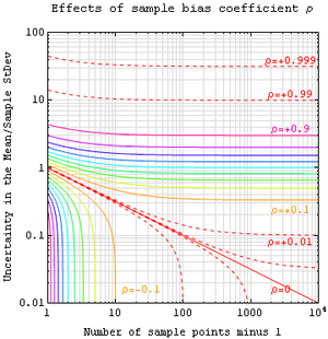
If values of the measured quantity A are not statistically independent but have been obtained from known locations in parameter space x, an unbiased estimate of the true standard error of the mean (actually a correction on the standard deviation part) may be obtained by multiplying the calculated standard error of the sample by the factor f:

where the sample bias coefficient ρ is the widely used Prais-Winsten estimate of the autocorrelation-coefficient (a quantity between −1 and +1) for all sample point pairs. This approximate formula is for moderate to large sample sizes; the reference gives the exact formulas for any sample size, and can be applied to heavily autocorrelated time series like Wall Street stock quotes. Moreover, this formula works for positive and negative ρ alike.[10] See also unbiased estimation of standard deviation for more discussion.
Relative standard error
The relative standard error of a sample mean is the standard error divided by the mean and expressed as a percentage. It can only be calculated if the mean is a non-zero value.
As an example of the use of the relative standard error, consider two surveys of household income that both result in a sample mean of $50,000. If one survey has a standard error of $10,000 and the other has a standard error of $5,000, then the relative standard errors are 20% and 10% respectively. The survey with the lower relative standard error can be said to have a more precise measurement, since it has proportionately less sampling variation around the mean. In fact, data organizations often set reliability standards that their data must reach before publication. For example, the U.S. National Center for Health Statistics typically does not report an estimated mean if its relative standard error exceeds 30%. (NCHS also typically requires at least 30 observations – if not more – for an estimate to be reported.)[11]
See also
- Coefficient of variation
- Illustration of the central limit theorem
- Probable error
- Standard error of the weighted mean
- Sample mean and sample covariance
- Variance
References
- ↑ Everitt, B.S. (2003) The Cambridge Dictionary of Statistics, CUP. ISBN 0-521-81099-X
- ↑ Kenney, J. and Keeping, E.S. (1963) Mathematics of Statistics, van Nostrand, p. 187
- ↑ Zwillinger D. (1995), Standard Mathematical Tables and Formulae, Chapman&Hall/CRC. ISBN 0-8493-2479-3 p. 626
- 1 2 Dietz, Davidl; Barr, Christopher; Çetinkaya-Rundel, Mine (2012), OpenIntro Statistics (Second ed.), openintro.org
- ↑ T.P. Hutchinson, Essentials of statistical methods in 41 pages
- ↑ Gurland, J; Tripathi RC (1971). "A simple approximation for unbiased estimation of the standard deviation". American Statistician. American Statistical Association. 25 (4): 30–32. doi:10.2307/2682923. JSTOR 2682923.
- ↑ Sokal and Rohlf (1981) Biometry: Principles and Practice of Statistics in Biological Research , 2nd ed. ISBN 0-7167-1254-7 , p 53
- ↑ Barde, M. (2012). "What to use to express the variability of data: Standard deviation or standard error of mean?". Perspect Clin Res. 3 (3): 113–116. doi:10.4103/2229-3485.100662.
- ↑ Isserlis, L. (1918). "On the value of a mean as calculated from a sample". Journal of the Royal Statistical Society. Blackwell Publishing. 81 (1): 75–81. doi:10.2307/2340569. JSTOR 2340569. (Equation 1)
- ↑ James R. Bence (1995) Analysis of short time series: Correcting for autocorrelation. Ecology 76(2): 628 – 639.
- ↑ Klein, RJ. "Healthy People 2010 criteria for data suppression" (PDF). Statistical Notes. Hyattsville, MD: U.S. National Center for Health Statistics (24). Retrieved 17 July 2014.
| |||||||||||||||||||||||||||||||||||||||||||||
| |||||||||||||||||||||||||||||||||||||||||||||
| |||||||||||||||||||||||||||||||||||||||||||||
| |||||||||||||||||||||||||||||||||||||||||||||
| |||||||||||||||||||||||||||||||||||||||||||||
| |||||||||||||||||||||||||||||||||||||||||||||
| |||||||||||||||||||||||||||||||||||||||||||||