Autocorrelation
Autocorrelation, also known as serial correlation, is the correlation of a signal with itself at different points in time. Informally, it is the similarity between observations as a function of the time lag between them. It is a mathematical tool for finding repeating patterns, such as the presence of a periodic signal obscured by noise, or identifying the missing fundamental frequency in a signal implied by its harmonic frequencies. It is often used in signal processing for analyzing functions or series of values, such as time domain signals.
Unit root processes, trend stationary processes, autoregressive processes, and moving average processes are specific forms of processes with autocorrelation.
Definitions
Different fields of study define autocorrelation differently, and not all of these definitions are equivalent. In some fields, the term is used interchangeably with autocovariance.
Statistics
In statistics, the autocorrelation of a random process is the correlation between values of the process at different times, as a function of the two times or of the time lag. Let X be a stochastic process, and t be any point in time. (t may be an integer for a discrete-time process or a real number for a continuous-time process.) Then Xt is the value (or realization) produced by a given run of the process at time t. Suppose that the process has mean μt and variance σt2 at time t, for each t. Then the definition of the autocorrelation between times s and t is
![R(s,t)={\frac {\operatorname {E} [(X_{t}-\mu _{t})(X_{s}-\mu _{s})]}{\sigma _{t}\sigma _{s}}}\,,](../I/m/61cd0217dfa828f09acfd38f88aad6936f038fe0.svg)
where "E" is the expected value operator. Note that this expression is not well-defined for all-time series or processes, because the mean may not exist, or the variance may be zero (for a constant process) or infinite (for processes with distribution lacking well-behaved moments, such as certain types of power law). If the function R is well-defined, its value must lie in the range [−1, 1], with 1 indicating perfect correlation and −1 indicating perfect anti-correlation.
If Xt is a wide-sense stationary process then the mean μ and the variance σ2 are time-independent, and further the autocorrelation depends only on the lag between t and s: the correlation depends only on the time-distance between the pair of values but not on their position in time. This further implies that the autocorrelation can be expressed as a function of the time-lag, and that this would be an even function of the lag τ = s − t. This gives the more familiar form
![R(\tau )={\frac {\operatorname {E} [(X_{t}-\mu )(X_{t+\tau }-\mu )]}{\sigma ^{2}}},\,](../I/m/6f5a7621bdc7c05989a3cb9e4effbc468e064b1b.svg)
and the fact that this is an even function can be stated as

It is common practice in some disciplines, other than statistics and time series analysis, to drop the normalization by σ2 and use the term "autocorrelation" interchangeably with "autocovariance". However, the normalization is important both because the interpretation of the autocorrelation as a correlation provides a scale-free measure of the strength of statistical dependence, and because the normalization has an effect on the statistical properties of the estimated autocorrelations.
Signal processing
In signal processing, the above definition is often used without the normalization, that is, without subtracting the mean and dividing by the variance. When the autocorrelation function is normalized by mean and variance, it is sometimes referred to as the autocorrelation coefficient.[1]
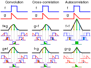
Given a signal , the continuous autocorrelation is most often defined as the continuous cross-correlation integral of with itself, at lag .


where represents the complex conjugate, is a function which manipulates the function and is defined as and represents convolution.


For a real function, .

Note that the parameter in the integral is a dummy variable and is only necessary to calculate the integral. It has no specific meaning.

The discrete autocorrelation at lag for a discrete signal is


The above definitions work for signals that are square integrable, or square summable, that is, of finite energy. Signals that "last forever" are treated instead as random processes, in which case different definitions are needed, based on expected values. For wide-sense-stationary random processes, the autocorrelations are defined as
![R_{ff}(\tau )=\operatorname {E} \left[f(t){\overline {f}}(t-\tau )\right]](../I/m/5be7d2e4d8c504d0c68e3a4b36687bed7cd60f5d.svg)
![R_{yy}(l)=\operatorname {E} \left[y(n)\,{\overline {y}}(n-l)\right].](../I/m/fd64b05417ffd5c20bd0f5b65effab1758839002.svg)
For processes that are not stationary, these will also be functions of , or .


For processes that are also ergodic, the expectation can be replaced by the limit of a time average. The autocorrelation of an ergodic process is sometimes defined as or equated to[1]


These definitions have the advantage that they give sensible well-defined single-parameter results for periodic functions, even when those functions are not the output of stationary ergodic processes.
Alternatively, signals that last forever can be treated by a short-time autocorrelation function analysis, using finite time integrals. (See short-time Fourier transform for a related process.)
Multi-dimensional autocorrelation is defined similarly. For example, in three dimensions the autocorrelation of a square-summable discrete signal would be

When mean values are subtracted from signals before computing an autocorrelation function, the resulting function is usually called an auto-covariance function.
Properties
In the following, we will describe properties of one-dimensional autocorrelations only, since most properties are easily transferred from the one-dimensional case to the multi-dimensional cases.
- A fundamental property of the autocorrelation is symmetry, , which is easy to prove from the definition. In the continuous case,

- the autocorrelation is an even function
- when is a real function,

- and the autocorrelation is a Hermitian function
- when is a complex function.

- The continuous autocorrelation function reaches its peak at the origin, where it takes a real value, i.e. for any delay , . This is a consequence of the rearrangement inequality. The same result holds in the discrete case.
- The autocorrelation of a periodic function is, itself, periodic with the same period.
- The autocorrelation of the sum of two completely uncorrelated functions (the cross-correlation is zero for all ) is the sum of the autocorrelations of each function separately.
- Since autocorrelation is a specific type of cross-correlation, it maintains all the properties of cross-correlation.
- The autocorrelation of a continuous-time white noise signal will have a strong peak (represented by a Dirac delta function) at and will be absolutely 0 for all other .
- The Wiener–Khinchin theorem relates the autocorrelation function to the power spectral density via the Fourier transform:


- For real-valued functions, the symmetric autocorrelation function has a real symmetric transform, so the Wiener–Khinchin theorem can be re-expressed in terms of real cosines only:


Efficient computation
For data expressed as a discrete sequence, it is frequently necessary to compute the autocorrelation with high computational efficiency. A brute force method based on the signal processing definition can be used when the signal size is small. For example, to calculate the autocorrelation of the real signal sequence (i.e. , and for all other values of i) by hand, we first recognize that the definition just given is same as the "usual" multiplication, but with right shifts, where each vertical addition gives the autocorrelation for particular lag values:


Thus the required autocorrelation sequence is , where and the autocorrelation for other lag values being zero. In this calculation we do not perform the carry-over operation during addition as is usual in normal multiplication. Note that we can halve the number of operations required by exploiting the inherent symmetry of the autocorrelation. If the signal happens to be periodic, i.e. then we get a circular autocorrelation (similar to circular convolution) where the left and right tails of the previous autocorrelation sequence will overlap and give which has the same period as the signal sequence The procedure can be regarded as an application of the convolution property of z-transform of a discrete signal.


While the brute force algorithm is order n2, several efficient algorithms exist which can compute the autocorrelation in order n log(n). For example, the Wiener–Khinchin theorem allows computing the autocorrelation from the raw data X(t) with two Fast Fourier transforms (FFT):[2]
![{\displaystyle {\begin{aligned}F_{R}(f)&=\operatorname {FFT} [X(t)]\\S(f)&=F_{R}(f)F_{R}^{*}(f)\\R(\tau )&=\operatorname {IFFT} [S(f)]\end{aligned}}}](../I/m/41ba8c3c366062d1c22b4ad97968f52961a40e82.svg)
where IFFT denotes the inverse Fast Fourier transform. The asterisk denotes complex conjugate.
Alternatively, a multiple τ correlation can be performed by using brute force calculation for low τ values, and then progressively binning the X(t) data with a logarithmic density to compute higher values, resulting in the same n log(n) efficiency, but with lower memory requirements.[3][4]
Estimation
For a discrete process with known mean and variance for which we observe observations , an estimate of the autocorrelation may be obtained as


for any positive integer . When the true mean and variance are known, this estimate is unbiased. If the true mean and variance of the process are not known there are a several possibilities:


- If and are replaced by the standard formulae for sample mean and sample variance, then this is a biased estimate.
- A periodogram-based estimate replaces in the above formula with . This estimate is always biased; however, it usually has a smaller mean square error.[5][6]
- Other possibilities derive from treating the two portions of data and separately and calculating separate sample means and/or sample variances for use in defining the estimate.


The advantage of estimates of the last type is that the set of estimated autocorrelations, as a function of , then form a function which is a valid autocorrelation in the sense that it is possible to define a theoretical process having exactly that autocorrelation. Other estimates can suffer from the problem that, if they are used to calculate the variance of a linear combination of the 's, the variance calculated may turn out to be negative.


Regression analysis
In regression analysis using time series data, autocorrelation in a variable of interest is typically modeled either with an autoregressive model (AR), a moving average model (MA), their combination as an autoregressive moving average model (ARMA), or an extension of the latter called an autoregressive integrated moving average model (ARIMA). With multiple interrelated data series, vector autoregression (VAR) or its extensions are used.
In ordinary least squares (OLS), the adequacy of a model specification can be checked in part by establishing whether there is autocorrelation of the regression residuals. Problematic autocorrelation of the errors, which themselves are unobserved, can generally be detected because it produces autocorrelation in the observable residuals. (Errors are also known as "error terms" in econometrics.) Autocorrelation of the errors violates the ordinary least squares assumption that the error terms are uncorrelated, meaning that the Gauss Markov theorem does not apply, and that OLS estimators are no longer the Best Linear Unbiased Estimators (BLUE). While it does not bias the OLS coefficient estimates, the standard errors tend to be underestimated (and the t-scores overestimated) when the autocorrelations of the errors at low lags are positive.
The traditional test for the presence of first-order autocorrelation is the Durbin–Watson statistic or, if the explanatory variables include a lagged dependent variable, Durbin's h statistic. The Durbin-Watson can be linearly mapped however to the Pearson correlation between values and their lags.[7] A more flexible test, covering autocorrelation of higher orders and applicable whether or not the regressors include lags of the dependent variable, is the Breusch–Godfrey test. This involves an auxiliary regression, wherein the residuals obtained from estimating the model of interest are regressed on (a) the original regressors and (b) k lags of the residuals, where k is the order of the test. The simplest version of the test statistic from this auxiliary regression is TR2, where T is the sample size and R2 is the coefficient of determination. Under the null hypothesis of no autocorrelation, this statistic is asymptotically distributed as with k degrees of freedom.

Responses to nonzero autocorrelation include generalized least squares and the Newey–West HAC estimator (Heteroskedasticity and Autocorrelation Consistent).[8]
In the estimation of a moving average model (MA), the autocorrelation function is used to determine the appropriate number of lagged error terms to be included. This is based on the fact that for an MA process of order q, we have , for , and , for .


Applications
- Autocorrelation analysis is used heavily in fluorescence correlation spectroscopy.
- Another application of autocorrelation is the measurement of optical spectra and the measurement of very-short-duration light pulses produced by lasers, both using optical autocorrelators.
- Autocorrelation is used to analyze dynamic light scattering data, which notably enables determination of the particle size distributions of nanometer-sized particles or micelles suspended in a fluid. A laser shining into the mixture produces a speckle pattern that results from the motion of the particles. Autocorrelation of the signal can be analyzed in terms of the diffusion of the particles. From this, knowing the viscosity of the fluid, the sizes of the particles can be calculated.
- The small-angle X-ray scattering intensity of a nanostructured system is the Fourier transform of the spatial autocorrelation function of the electron density.
- In optics, normalized autocorrelations and cross-correlations give the degree of coherence of an electromagnetic field.
- In signal processing, autocorrelation can give information about repeating events like musical beats (for example, to determine tempo) or pulsar frequencies, though it cannot tell the position in time of the beat. It can also be used to estimate the pitch of a musical tone.
- In music recording, autocorrelation is used as a pitch detection algorithm prior to vocal processing, as a distortion effect or to eliminate undesired mistakes and inaccuracies.[9]
- Autocorrelation in space rather than time, via the Patterson function, is used by X-ray diffractionists to help recover the "Fourier phase information" on atom positions not available through diffraction alone.
- In statistics, spatial autocorrelation between sample locations also helps one estimate mean value uncertainties when sampling a heterogeneous population.
- The SEQUEST algorithm for analyzing mass spectra makes use of autocorrelation in conjunction with cross-correlation to score the similarity of an observed spectrum to an idealized spectrum representing a peptide.
- In astrophysics, auto-correlation is used to study and characterize the spatial distribution of galaxies in the universe and in multi-wavelength observations of low mass X-ray binaries.
- In panel data, spatial autocorrelation refers to correlation of a variable with itself through space.
- In analysis of Markov chain Monte Carlo data, autocorrelation must be taken into account for correct error determination.
- In geosciences (specifically in geophysics) it can be used to compute an autocorrelation seismic attribute, out of a 3D seismic survey of the underground.
- In medical ultrasound imaging, autocorrelation is used to visualize blood flow.
Serial dependence
Serial dependence is closely linked to the notion of autocorrelation, but represents a distinct concept (see Correlation and dependence). In particular, it is possible to have serial dependence but no (linear) correlation, or a measured correlation but no actual statistical dependence. In some fields however, the two terms are used as synonyms.
Random variables in a time series have serial dependence if the value at some time t in the series is statistically dependent on the value at another time s. A series is serially independent if there is no dependence between any pair.
If a time series {Xt} is stationary, then statistical dependence between the pair (Xt , Xs) would imply that there is statistical dependence between all pairs of values at the same lag s−t.
See also
- Autocorrelation matrix
- Autocorrelation technique
- Autocorrelator
- Correlation function
- Correlogram
- Covariance mapping
- Cross-correlation
- Galton's problem
- Partial autocorrelation function
- Fluorescence correlation spectroscopy
- Optical autocorrelation
- Pitch detection algorithm
- Triple correlation
- Variance
- CUSUM
- Cochrane–Orcutt estimation (transformation for autocorrelated error terms)
- Prais–Winsten transformation
- Scaled Correlation
- Unbiased estimation of standard deviation#Effect of autocorrelation (serial correlation)
References
- 1 2 Dunn, Patrick F. (2005). Measurement and Data Analysis for Engineering and Science. New York: McGraw–Hill. ISBN 0-07-282538-3.
- ↑ Box, G. E. P.; Jenkins, G. M.; Reinsel, G. C. (1994). Time Series Analysis: Forecasting and Control (3rd ed.). Upper Saddle River, NJ: Prentice–Hall. ISBN 0130607746.
- ↑ Frenkel, D.; Smit, B. (2002). "chap. 4.4.2". Understanding Molecular Simulation (2nd ed.). London: Academic Press. ISBN 0122673514.
- ↑ Colberg, P.; Höfling, F. (2011). "Highly accelerated simulations of glassy dynamics using GPUs: caveats on limited floating-point precision". Comp. Phys. Comm. 182 (5): 1120–1129. doi:10.1016/j.cpc.2011.01.009.
- ↑ Priestley, M. B. (1982). Spectral analysis and time series. London, New York: Academic Press. ISBN 0125649010.
- ↑ Percival, Donald B.; Andrew T. Walden (1993). Spectral Analysis for Physical Applications: Multitaper and Conventional Univariate Techniques. Cambridge University Press. pp. 190–195. ISBN 0-521-43541-2.
- ↑ "Statistical Ideas: Serial correlation techniques".
- ↑ Baum, Christopher F. (2006). An Introduction to Modern Econometrics Using Stata. Stata Press. ISBN 1-59718-013-0.
- ↑ Tyrangiel, Josh (2009-02-05). "Auto-Tune: Why Pop Music Sounds Perfect". Time Magazine.
Further reading
- Kmenta, Jan (1986). Elements of Econometrics (Second ed.). New York: Macmillan. pp. 298–334. ISBN 0-02-365070-2.
- Verbeek, Marno (2012). A Guide to Modern Econometrics (Fourth ed.). Chichester: John Wiley. pp. 112–116. ISBN 978-1-119-95167-4.
- Mojtaba Soltanalian, and Petre Stoica. "Computational design of sequences with good correlation properties." IEEE Transactions on Signal Processing, 60.5 (2012): 2180-2193.
- Solomon W. Golomb, and Guang Gong. Signal design for good correlation: for wireless communication, cryptography, and radar. Cambridge University Press, 2005.
External links
- Autocorrelation articles in Comp.DSP (DSP usenet group).
- GPU accelerated calculation of autocorrelation function.
- Econometrics lecture (topic: autocorrelation) on YouTube by Mark Thoma
- Autocorrelation Time Series data by itfeature
| |||||||||||||||||||||||||||||||||||||||||||||
| |||||||||||||||||||||||||||||||||||||||||||||
| |||||||||||||||||||||||||||||||||||||||||||||
| |||||||||||||||||||||||||||||||||||||||||||||
| |||||||||||||||||||||||||||||||||||||||||||||
| |||||||||||||||||||||||||||||||||||||||||||||
| |||||||||||||||||||||||||||||||||||||||||||||