Maximum spacing estimation
In statistics, maximum spacing estimation (MSE or MSP), or maximum product of spacing estimation (MPS), is a method for estimating the parameters of a univariate statistical model.[1] The method requires maximization of the geometric mean of spacings in the data, which are the differences between the values of the cumulative distribution function at neighbouring data points.
The concept underlying the method is based on the probability integral transform, in that a set of independent random samples derived from any random variable should on average be uniformly distributed with respect to the cumulative distribution function of the random variable. The MPS method chooses the parameter values that make the observed data as uniform as possible, according to a specific quantitative measure of uniformity.
One of the most common methods for estimating the parameters of a distribution from data, the method of maximum likelihood (MLE), can break down in various cases, such as involving certain mixtures of continuous distributions.[2] In these cases the method of maximum spacing estimation may be successful.
Apart from its use in pure mathematics and statistics, the trial applications of the method have been reported using data from fields such as hydrology,[3] econometrics,[4] magnetic resonance imaging,[5] and others.[6]
History and usage
The MSE method was derived independently by Russel Cheng and Nik Amin at the University of Wales Institute of Science and Technology, and Bo Ranneby at the Swedish University of Agricultural Sciences.[2] The authors explained that due to the probability integral transform at the true parameter, the “spacing” between each observation should be uniformly distributed. This would imply that the difference between the values of the cumulative distribution function at consecutive observations should be equal. This is the case that maximizes the geometric mean of such spacings, so solving for the parameters that maximize the geometric mean would achieve the “best” fit as defined this way. Ranneby (1984) justified the method by demonstrating that it is an estimator of the Kullback–Leibler divergence, similar to maximum likelihood estimation, but with more robust properties for various classes of problems.
There are certain distributions, especially those with three or more parameters, whose likelihoods may become infinite along certain paths in the parameter space. Using maximum likelihood to estimate these parameters often breaks down, with one parameter tending to the specific value that causes the likelihood to be infinite, rendering the other parameters inconsistent. The method of maximum spacings, however, being dependent on the difference between points on the cumulative distribution function and not individual likelihood points, does not have this issue, and will return valid results over a much wider array of distributions.[1]
The distributions that tend to have likelihood issues are often those used to model physical phenomena. Hall & al. (2004) seek to analyze flood alleviation methods, which requires accurate models of river flood effects. The distributions that better model these effects are all three-parameter models, which suffer from the infinite likelihood issue described above, leading to Hall’s investigation of the maximum spacing procedure. Wong & Li (2006), when comparing the method to maximum likelihood, use various data sets ranging from a set on the oldest ages at death in Sweden between 1905 and 1958 to a set containing annual maximum wind speeds.
Definition
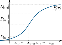
Given an iid random sample {x1, …, xn} of size n from a univariate distribution with the cumulative distribution function F(x;θ0), where θ0 ∈ Θ is an unknown parameter to be estimated, let {x(1), …, x(n)} be the corresponding ordered sample, that is the result of sorting of all observations from smallest to largest. For convenience also denote x(0) = −∞ and x(n+1) = +∞.
Define the spacings as the “gaps” between the values of the distribution function at adjacent ordered points:[7]

Then the maximum spacing estimator of θ0 is defined as a value that maximizes the logarithm of the geometric mean of sample spacings:
![{\hat {\theta }}={\underset {\theta \in \Theta }{\operatorname {arg\,max} }}\;S_{n}(\theta ),\quad {\text{where }}\ S_{n}(\theta )=\ln \!\!{\sqrt[{n+1}]{D_{1}D_{2}\cdots D_{n+1}}}={\frac {1}{n+1}}\sum _{i=1}^{n+1}\ln {D_{i}}(\theta ).](../I/m/9a31b5ecd6b17eba0ab4543bd2d844d706d1f573.svg)
By the inequality of arithmetic and geometric means, function Sn(θ) is bounded from above by −ln(n+1), and thus the maximum has to exist at least in the supremum sense.
Note that some authors define the function Sn(θ) somewhat differently. In particular, Ranneby (1984) multiplies each Di by a factor of (n+1), whereas Cheng & Stephens (1989) omit the 1⁄n+1 factor in front of the sum and add the “−” sign in order to turn the maximization into minimization. As these are constants with respect to θ, the modifications do not alter the location of the maximum of the function Sn.
Examples
This section presents two examples of calculating the maximum spacing estimator.
Example 1
Suppose two values x(1) = 2, x(2) = 4 were sampled from the exponential distribution F(x;λ) = 1 − e−xλ, x ≥ 0 with unknown parameter λ > 0. In order to construct the MSE we have to first find the spacings:
| i | F(x(i)) | F(x(i−1)) | Di = F(x(i)) − F(x(i−1)) |
|---|---|---|---|
| 1 | 1 − e−2λ | 0 | 1 − e−2λ |
| 2 | 1 − e−4λ | 1 − e−2λ | e−2λ − e−4λ |
| 3 | 1 | 1 − e−4λ | e−4λ |
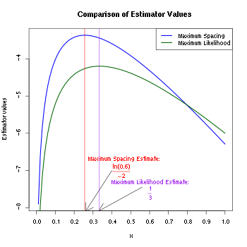
The process continues by finding the λ that maximizes the geometric mean of the “difference” column. Using the convention that ignores taking the (n+1)st root, this turns into the maximization of the following product: (1 − e−2λ) · (e−2λ − e−4λ) · (e−4λ). Letting μ = e−2λ, the problem becomes finding the maximum of μ5−2μ4+μ3. Differentiating, the μ has to satisfy 5μ4−8μ3+3μ2 = 0. This equation has roots 0, 0.6, and 1. As μ is actually e−2λ, it has to be greater than zero but less than one. Therefore, the only acceptable solution is

which corresponds to an exponential distribution with a mean of 1⁄λ ≈ 3.915. For comparison, the maximum likelihood estimate of λ is the inverse of the sample mean, 3, so λMLE = ⅓ ≈ 0.333.
Example 2
Suppose {x(1), …, x(n)} is the ordered sample from a uniform distribution U(a,b) with unknown endpoints a and b. The cumulative distribution function is F(x;a,b) = (x−a)/(b−a) when x∈[a,b]. Therefore individual spacings are given by

Calculating the geometric mean and then taking the logarithm, statistic Sn will be equal to

Here only the first three terms depend on the parameters a and b. Differentiating with respect to those parameters and solving the resulting linear system, the maximum spacing estimates will be

These are known to be the uniformly minimum variance unbiased (UMVU) estimators for the continuous uniform distribution.[1] In comparison, the maximum likelihood estimates for this problem and are biased and have higher mean-squared error.


Properties
Consistency and efficiency


The maximum spacing estimator is a consistent estimator in that it converges in probability to the true value of the parameter, θ0, as the sample size increases to infinity.[2] The consistency of maximum spacing estimation holds under much more general conditions than for maximum likelihood estimators. In particular, in cases where the underlying distribution is J-shaped, maximum likelihood will fail where MSE succeeds.[1] An example of a J-shaped density is the Weibull distribution, specifically a shifted Weibull, with a shape parameter less than 1. The density will tend to infinity as x approaches the location parameter rendering estimates of the other parameters inconsistent.
Maximum spacing estimators are also at least as asymptotically efficient as maximum likelihood estimators, where the latter exist. However, MSEs may exist in cases where MLEs do not.[1]
Sensitivity
Maximum spacing estimators are sensitive to closely spaced observations, and especially ties.[8] Given

we get

When the ties are due to multiple observations, the repeated spacings (those that would otherwise be zero) should be replaced by the corresponding likelihood.[1] That is, one should substitute for , as


since .

When ties are due to rounding error, Cheng & Stephens (1989) suggest another method to remove the effects.[note 1] Given r tied observations from xi to xi+r−1, let δ represent the round-off error. All of the true values should then fall in the range . The corresponding points on the distribution should now fall between and . Cheng and Stephens suggest assuming that the rounded values are uniformly spaced in this interval, by defining


The MSE method is also sensitive to secondary clustering.[8] One example of this phenomenon is when a set of observations is thought to come from a single normal distribution, but in fact comes from a mixture normals with different means. A second example is when the data is thought to come from an exponential distribution, but actually comes from a gamma distribution. In the latter case, smaller spacings may occur in the lower tail. A high value of M(θ) would indicate this secondary clustering effect, and suggesting a closer look at the data is required.[8]
Goodness of fit
The statistic Sn(θ) is also a form of Moran or Moran-Darling statistic, M(θ), which can be used to test goodness of fit.[note 2] It has been shown that the statistic, when defined as

is asymptotically normal, and that a chi-squared approximation exists for small samples.[8] In the case where we know the true parameter , Cheng & Stephens (1989) show that the statistic has a normal distribution with


where γ is the Euler–Mascheroni constant which is approximately 0.57722.[note 3]
The distribution can also be approximated by that of , where

- ,

in which

and where follows a chi-squared distribution with degrees of freedom. Therefore, to test the hypothesis that a random sample of values comes from the distribution , the statistic can be calculated. Then should be rejected with significance if the value is greater than the critical value of the appropriate chi-squared distribution.[8]


Where θ0 is being estimated by , Cheng & Stephens (1989) showed that has the same asymptotic mean and variance as in the known case. However, the test statistic to be used requires the addition of a bias correction term and is:


where is the number of parameters in the estimate.

Generalized maximum spacing
Alternate measures and spacings
Ranneby & Ekström (1997) generalized the MSE method to approximate other measures besides the Kullback–Leibler measure. Ekström (1997) further expanded the method to investigate properties of estimators using higher order spacings, where an m-order spacing would be defined as .

Multivariate distributions
Ranneby & al. (2005) discuss extended maximum spacing methods to the multivariate case. As there is no natural order for , they discuss two alternative approaches: a geometric approach based on Dirichlet cells and a probabilistic approach based on a “nearest neighbor ball” metric.

See also
Notes
- ↑ There appear to be some minor typographical errors in the paper. For example, in section 4.2, equation (4.1), the rounding replacement for , should not have the log term. In section 1, equation (1.2), is defined to be the spacing itself, and is the negative sum of the logs of . If is logged at this step, the result is always ≤ 0, as the difference between two adjacent points on a cumulative distribution is always ≤ 1, and strictly < 1 unless there are only two points at the bookends. Also, in section 4.3, on page 392, calculation shows that it is the variance which has MPS estimate of 6.87, not the standard deviation . – Editor
- ↑ The literature refers to related statistics as Moran or Moran-Darling statistics. For example, Cheng & Stephens (1989) analyze the form where is defined as above. Wong & Li (2006) use the same form as well. However, Beirlant & al. (2001) uses the form , with the additional factor of inside the logged summation. The extra factors will make a difference in terms of the expected mean and variance of the statistic. For consistency, this article will continue to use the Cheng & Amin/Wong & Li form. -- Editor
- ↑ Wong & Li (2006) leave out the Euler–Mascheroni constant from their description. -- Editor


References
Works cited
- Anatolyev, Stanislav; Kosenok, Grigory (2005). "An alternative to maximum likelihood based on spacings" (PDF). Econometric Theory. 21 (2): 472–476. doi:10.1017/S0266466605050255. Retrieved 2009-01-21.
- Beirlant, J.; Dudewicz, E.J.; Györfi, L.; van der Meulen, E.C. (1997). "Nonparametric entropy estimation: an overview" (PDF). International Journal of Mathematical and Statistical Sciences. 6 (1): 17–40. ISSN 1055-7490. Archived from the original (PDF) on May 5, 2005. Retrieved 2008-12-31. Note: linked paper is an updated 2001 version.
- Cheng, R.C.H.; Amin, N.A.K. (1983). "Estimating parameters in continuous univariate distributions with a shifted origin". Journal of the Royal Statistical Society, Series B. 45 (3): 394–403. ISSN 0035-9246. JSTOR 2345411.
- Cheng, R.C.H; Stephens, M. A. (1989). "A goodness-of-fit test using Moran's statistic with estimated parameters". Biometrika. 76 (2): 386–392. doi:10.1093/biomet/76.2.385.
- Ekström, Magnus (1997). "Generalized maximum spacing estimates". University of Umeå, Department of Mathematics. 6. ISSN 0345-3928. Archived from the original on February 14, 2007. Retrieved 2008-12-30.
- Hall, M.J.; van den Boogaard, H.F.P.; Fernando, R.C.; Mynett, A.E. (2004). "The construction of confidence intervals for frequency analysis using resampling techniques" (PDF). Hydrology and Earth System Sciences. 8 (2): 235–246. doi:10.5194/hess-8-235-2004. ISSN 1027-5606. Retrieved 2009-01-21.
- Pieciak, Tomasz (2014). The maximum spacing noise estimation in single-coil background MRI data (PDF). IEEE International Conference on Image Processing. Paris. pp. 1743–1747. Retrieved 2015-07-07.
- Pyke, Ronald (1965). "Spacings". Journal of the Royal Statistical Society, Series B. 27 (3): 395–449. ISSN 0035-9246. JSTOR 2345793.
- Ranneby, Bo (1984). "The maximum spacing method. An estimation method related to the maximum likelihood method". Scandinavian Journal of Statistics. 11 (2): 93–112. ISSN 0303-6898. JSTOR 4615946.
- Ranneby, Bo; Ekström, Magnus (1997). "Maximum spacing estimates based on different metrics". University of Umeå, Department of Mathematics. 5. ISSN 0345-3928. Archived from the original on February 14, 2007. Retrieved 2008-12-30.
- Ranneby, Bo; Jammalamadakab, S. Rao; Teterukovskiy, Alex (2005). "The maximum spacing estimation for multivariate observations" (PDF). Journal of Statistical Planning and Inference. 129 (1–2): 427–446. doi:10.1016/j.jspi.2004.06.059. Retrieved 2008-12-31.
- Wong, T.S.T; Li, W.K. (2006). "A note on the estimation of extreme value distributions using maximum product of spacings". Time series and related topics: in memory of Ching-Zong Wei. Beachwood, Ohio: Institute of Mathematical Statistic. pp. 272–283. arXiv:math/0702830v1
 . doi:10.1214/074921706000001102.
| |||||||||||||||||||||||||||||||||||||||||||||
| |||||||||||||||||||||||||||||||||||||||||||||
| |||||||||||||||||||||||||||||||||||||||||||||
| |||||||||||||||||||||||||||||||||||||||||||||
| |||||||||||||||||||||||||||||||||||||||||||||
| |||||||||||||||||||||||||||||||||||||||||||||
| |||||||||||||||||||||||||||||||||||||||||||||