Bayesian inference

Bayesian inference is a method of statistical inference in which Bayes' theorem is used to update the probability for a hypothesis as more evidence or information becomes available. Bayesian inference is an important technique in statistics, and especially in mathematical statistics. Bayesian updating is particularly important in the dynamic analysis of a sequence of data. Bayesian inference has found application in a wide range of activities, including science, engineering, philosophy, medicine, sport, and law. In the philosophy of decision theory, Bayesian inference is closely related to subjective probability, often called "Bayesian probability".

Introduction to Bayes' rule

A geometric visualisation of Bayes' theorem. In the table, the values w, x, y and z give the relative weights of each corresponding condition and case. The figures denote the cells of the table involved in each metric, the probability being the fraction of each figure that is shaded. This shows that P(A|B) P(B) = P(B|A) P(A) i.e. P(A|B) = P(B|A) P(A)/P(B) . Similar reasoning can be used to show that P(Ā|B) = P(B|Ā) P(Ā)/P(B) etc.

Formal

Bayesian inference derives the posterior probability as a consequence of two antecedents, a prior probability and a "likelihood function" derived from a statistical model for the observed data. Bayesian inference computes the posterior probability according to Bayes' theorem:

$P(H\mid E)={\frac {P(E\mid H)\cdot P(H)}{P(E)}}$

where

• $\textstyle \mid$ means "event conditional on" (so that ${\displaystyle \textstyle (A\mid B)}$ means A given B).
• $\textstyle H$ stands for any hypothesis whose probability may be affected by data (called evidence below). Often there are competing hypotheses, and the task is to determine which is the most probable.
• the evidence $\textstyle E$ corresponds to new data that were not used in computing the prior probability.
• $\textstyle P(H)$, the prior probability, is the estimate of the probability of the hypothesis $\textstyle H$ before the data $\textstyle E$, the current evidence, is observed.
• $\textstyle P(H\mid E)$, the posterior probability, is the probability of $\textstyle H$ given $\textstyle E$, i.e., after $\textstyle E$ is observed. This is what we want to know: the probability of a hypothesis given the observed evidence.
• $\textstyle P(E\mid H)$ is the probability of observing $\textstyle E$ given $\textstyle H$. As a function of $\textstyle E$ with $\textstyle H$ fixed, this is the likelihood – it indicates the compatibility of the evidence with the given hypothesis. The likelihood function is a function of the evidence, $\textstyle E$, while the posterior probability is a function of the hypothesis, $\textstyle H$.
• $\textstyle P(E)$ is sometimes termed the marginal likelihood or "model evidence". This factor is the same for all possible hypotheses being considered (as is evident from the fact that the hypothesis $\textstyle H$ does not appear anywhere in the symbol, unlike for all the other factors), so this factor does not enter into determining the relative probabilities of different hypotheses.

For different values of $\textstyle H$, only the factors $\textstyle P(H)$ and $\textstyle P(E\mid H)$, both in the numerator, affect the value of $\textstyle P(H\mid E)$ – the posterior probability of a hypothesis is proportional to its prior probability (its inherent likeliness) and the newly acquired likelihood (its compatibility with the new observed evidence).

Bayes' rule can also be written as follows:

$P(H\mid E)={\frac {P(E\mid H)}{P(E)}}\cdot P(H)$

where the factor $\textstyle {\frac {P(E\mid H)}{P(E)}}$ can be interpreted as the impact of $E$ on the probability of $H$.

Informal

If the evidence does not match up with a hypothesis, one should reject the hypothesis. But if a hypothesis is extremely unlikely a priori, one should also reject it, even if the evidence does appear to match up. For example, if one does not know whether the newborn baby next door is a boy or a girl, the color of decorations on the crib in front of the door may support the hypothesis of one gender or the other; but if in front of that door, instead of the crib, a dog kennel is found, the posterior probability that the family next door gave birth to a dog remains small in spite of the "evidence", since one's prior belief in such a hypothesis was already extremely small.

The critical point about Bayesian inference, then, is that it provides a principled way of combining new evidence with prior beliefs, through the application of Bayes' rule. (Contrast this with frequentist inference, which relies only on the evidence as a whole, with no reference to prior beliefs.)

Furthermore, Bayes' rule can be applied iteratively: after observing some evidence, the resulting posterior probability can then be treated as a prior probability, and a new posterior probability computed from new evidence. This allows for Bayesian principles to be applied to various kinds of evidence, whether viewed all at once or over time. This procedure is termed "Bayesian updating".

Alternatives to Bayesian updating

Bayesian updating is widely used and computationally convenient. However, it is not the only updating rule that might be considered rational.

Ian Hacking noted that traditional "Dutch book" arguments did not specify Bayesian updating: they left open the possibility that non-Bayesian updating rules could avoid Dutch books. Hacking wrote^[1] "And neither the Dutch book argument, nor any other in the personalist arsenal of proofs of the probability axioms, entails the dynamic assumption. Not one entails Bayesianism. So the personalist requires the dynamic assumption to be Bayesian. It is true that in consistency a personalist could abandon the Bayesian model of learning from experience. Salt could lose its savour."

Indeed, there are non-Bayesian updating rules that also avoid Dutch books (as discussed in the literature on "probability kinematics" following the publication of Richard C. Jeffrey's rule, which applies Bayes' rule to the case where the evidence itself is assigned a probability.^[2] The additional hypotheses needed to uniquely require Bayesian updating have been deemed to be substantial, complicated, and unsatisfactory.^[3]

Formal description of Bayesian inference

Definitions

• $x$, a data point in general. This may in fact be a vector of values.
• $\theta$, the parameter of the data point's distribution, i.e., $x\sim p(x\mid \theta )$ . This may in fact be a vector of parameters.
• $\alpha$, the hyperparameter of the parameter, i.e., $\theta \sim p(\theta \mid \alpha )$ . This may in fact be a vector of hyperparameters.
• $\mathbf {X}$, a set of $n$ observed data points, i.e., $x_{1},\ldots ,x_{n}$.
• ${\tilde {x}}$, a new data point whose distribution is to be predicted.

Bayesian inference

• The prior distribution is the distribution of the parameter(s) before any data is observed, i.e. $p(\theta \mid \alpha )$ .
• The prior distribution might not be easily determined. In this case, we can use the Jeffreys prior to obtain the posterior distribution before updating them with newer observations.
• The sampling distribution is the distribution of the observed data conditional on its parameters, i.e. $p(\mathbf {X} \mid \theta )$ . This is also termed the likelihood, especially when viewed as a function of the parameter(s), sometimes written $\operatorname {L} (\theta \mid \mathbf {X} )=p(\mathbf {X} \mid \theta )$ .
• The marginal likelihood (sometimes also termed the evidence) is the distribution of the observed data marginalized over the parameter(s), i.e. $p(\mathbf {X} \mid \alpha )=\int _{\theta }p(\mathbf {X} \mid \theta )p(\theta \mid \alpha )\operatorname {d} \!\theta$ .
• The posterior distribution is the distribution of the parameter(s) after taking into account the observed data. This is determined by Bayes' rule, which forms the heart of Bayesian inference:

$p(\theta \mid \mathbf {X} ,\alpha )={\frac {p(\mathbf {X} \mid \theta )p(\theta \mid \alpha )}{p(\mathbf {X} \mid \alpha )}}\propto p(\mathbf {X} \mid \theta )p(\theta \mid \alpha )$

Note that this is expressed in words as "posterior is proportional to likelihood times prior", or sometimes as "posterior = likelihood times prior, over evidence".

Bayesian prediction

• The posterior predictive distribution is the distribution of a new data point, marginalized over the posterior:

$p({\tilde {x}}\mid \mathbf {X} ,\alpha )=\int _{\theta }p({\tilde {x}}\mid \theta )p(\theta \mid \mathbf {X} ,\alpha )\operatorname {d} \!\theta$

• The prior predictive distribution is the distribution of a new data point, marginalized over the prior:

$p({\tilde {x}}\mid \alpha )=\int _{\theta }p({\tilde {x}}\mid \theta )p(\theta \mid \alpha )\operatorname {d} \!\theta$

Bayesian theory calls for the use of the posterior predictive distribution to do predictive inference, i.e., to predict the distribution of a new, unobserved data point. That is, instead of a fixed point as a prediction, a distribution over possible points is returned. Only this way is the entire posterior distribution of the parameter(s) used. By comparison, prediction in frequentist statistics often involves finding an optimum point estimate of the parameter(s)—e.g., by maximum likelihood or maximum a posteriori estimation (MAP)—and then plugging this estimate into the formula for the distribution of a data point. This has the disadvantage that it does not account for any uncertainty in the value of the parameter, and hence will underestimate the variance of the predictive distribution.

(In some instances, frequentist statistics can work around this problem. For example, confidence intervals and prediction intervals in frequentist statistics when constructed from a normal distribution with unknown mean and variance are constructed using a Student's t-distribution. This correctly estimates the variance, due to the fact that (1) the average of normally distributed random variables is also normally distributed; (2) the predictive distribution of a normally distributed data point with unknown mean and variance, using conjugate or uninformative priors, has a student's t-distribution. In Bayesian statistics, however, the posterior predictive distribution can always be determined exactly—or at least, to an arbitrary level of precision, when numerical methods are used.)

Note that both types of predictive distributions have the form of a compound probability distribution (as does the marginal likelihood). In fact, if the prior distribution is a conjugate prior, and hence the prior and posterior distributions come from the same family, it can easily be seen that both prior and posterior predictive distributions also come from the same family of compound distributions. The only difference is that the posterior predictive distribution uses the updated values of the hyperparameters (applying the Bayesian update rules given in the conjugate prior article), while the prior predictive distribution uses the values of the hyperparameters that appear in the prior distribution.

Inference over exclusive and exhaustive possibilities

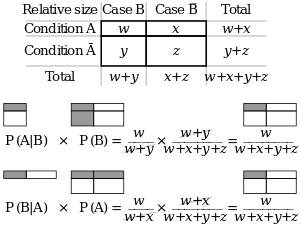
If evidence is simultaneously used to update belief over a set of exclusive and exhaustive propositions, Bayesian inference may be thought of as acting on this belief distribution as a whole.

General formulation

Diagram illustrating event space $\Omega$ in general formulation of Bayesian inference. Although this diagram shows discrete models and events, the continuous case may be visualized similarly using probability densities.

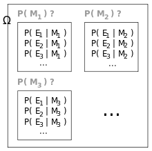
Suppose a process is generating independent and identically distributed events $E_{n}$, but the probability distribution is unknown. Let the event space $\Omega$ represent the current state of belief for this process. Each model is represented by event $M_{m}$. The conditional probabilities $P(E_{n}\mid M_{m})$ are specified to define the models. $P(M_{m})$ is the degree of belief in $M_{m}$. Before the first inference step, $\{P(M_{m})\}$ is a set of initial prior probabilities. These must sum to 1, but are otherwise arbitrary.

Suppose that the process is observed to generate $\textstyle E\in \{E_{n}\}$. For each $M\in \{M_{m}\}$, the prior $P(M)$ is updated to the posterior $P(M\mid E)$. From Bayes' theorem:^[4]

$P(M\mid E)={\frac {P(E\mid M)}{\sum _{m}{P(E\mid M_{m})P(M_{m})}}}\cdot P(M)$

Upon observation of further evidence, this procedure may be repeated.

Multiple observations

For a sequence of independent and identically distributed observations $\mathbf {E} =(e_{1},\dots ,e_{n})$, it can be shown by induction that repeated application of the above is equivalent to

$P(M\mid \mathbf {E} )={\frac {P(\mathbf {E} \mid M)}{\sum _{m}{P(\mathbf {E} \mid M_{m})P(M_{m})}}}\cdot P(M)$

Where

$P(\mathbf {E} \mid M)=\prod _{k}{P(e_{k}\mid M)}.$

Parametric formulation

By parameterizing the space of models, the belief in all models may be updated in a single step. The distribution of belief over the model space may then be thought of as a distribution of belief over the parameter space. The distributions in this section are expressed as continuous, represented by probability densities, as this is the usual situation. The technique is however equally applicable to discrete distributions.

Let the vector $\mathbf {\theta }$ span the parameter space. Let the initial prior distribution over $\mathbf {\theta }$ be $p(\mathbf {\theta } \mid \mathbf {\alpha } )$, where $\mathbf {\alpha }$ is a set of parameters to the prior itself, or hyperparameters. Let $\mathbf {E} =(e_{1},\dots ,e_{n})$ be a sequence of independent and identically distributed event observations, where all $e_{i}$ are distributed as $p(e\mid \mathbf {\theta } )$ for some $\mathbf {\theta }$. Bayes' theorem is applied to find the posterior distribution over $\mathbf {\theta }$:

${\begin{aligned}p(\mathbf {\theta } \mid \mathbf {E} ,\mathbf {\alpha } )&={\frac {p(\mathbf {E} \mid \mathbf {\theta } ,\mathbf {\alpha } )}{p(\mathbf {E} \mid \mathbf {\alpha } )}}\cdot p(\mathbf {\theta } \mid \mathbf {\alpha } )\\&={\frac {p(\mathbf {E} \mid \mathbf {\theta } ,\mathbf {\alpha } )}{\int _{\mathbf {\theta } }p(\mathbf {E} |\mathbf {\theta } ,\mathbf {\alpha } )p(\mathbf {\theta } \mid \mathbf {\alpha } )\,d\mathbf {\theta } }}\cdot p(\mathbf {\theta } \mid \mathbf {\alpha } )\end{aligned}}$

Where

$p(\mathbf {E} \mid \mathbf {\theta } ,\mathbf {\alpha } )=\prod _{k}p(e_{k}\mid \mathbf {\theta } )$

Mathematical properties

Interpretation of factor

$\textstyle {\frac {P(E\mid M)}{P(E)}}>1\Rightarrow \textstyle P(E\mid M)>P(E)$. That is, if the model were true, the evidence would be more likely than is predicted by the current state of belief. The reverse applies for a decrease in belief. If the belief does not change, $\textstyle {\frac {P(E\mid M)}{P(E)}}=1\Rightarrow \textstyle P(E\mid M)=P(E)$. That is, the evidence is independent of the model. If the model were true, the evidence would be exactly as likely as predicted by the current state of belief.

Cromwell's rule

If $P(M)=0$ then $P(M\mid E)=0$. If $P(M)=1$, then $P(M|E)=1$. This can be interpreted to mean that hard convictions are insensitive to counter-evidence.

The former follows directly from Bayes' theorem. The latter can be derived by applying the first rule to the event "not $M$" in place of "$M$", yielding "if $1-P(M)=0$, then $1-P(M\mid E)=0$", from which the result immediately follows.

Asymptotic behaviour of posterior

Consider the behaviour of a belief distribution as it is updated a large number of times with independent and identically distributed trials. For sufficiently nice prior probabilities, the Bernstein-von Mises theorem gives that in the limit of infinite trials, the posterior converges to a Gaussian distribution independent of the initial prior under some conditions firstly outlined and rigorously proven by Joseph L. Doob in 1948, namely if the random variable in consideration has a finite probability space. The more general results were obtained later by the statistician David A. Freedman who published in two seminal research papers in 1963 and 1965 when and under what circumstances the asymptotic behaviour of posterior is guaranteed. His 1963 paper treats, like Doob (1949), the finite case and comes to a satisfactory conclusion. However, if the random variable has an infinite but countable probability space (i.e., corresponding to a die with infinite many faces) the 1965 paper demonstrates that for a dense subset of priors the Bernstein-von Mises theorem is not applicable. In this case there is almost surely no asymptotic convergence. Later in the 1980s and 1990s Freedman and Persi Diaconis continued to work on the case of infinite countable probability spaces.^[5] To summarise, there may be insufficient trials to suppress the effects of the initial choice, and especially for large (but finite) systems the convergence might be very slow.

Conjugate priors

In parameterized form, the prior distribution is often assumed to come from a family of distributions called conjugate priors. The usefulness of a conjugate prior is that the corresponding posterior distribution will be in the same family, and the calculation may be expressed in closed form.

Estimates of parameters and predictions

It is often desired to use a posterior distribution to estimate a parameter or variable. Several methods of Bayesian estimation select measurements of central tendency from the posterior distribution.

For one-dimensional problems, a unique median exists for practical continuous problems. The posterior median is attractive as a robust estimator.^[6]

If there exists a finite mean for the posterior distribution, then the posterior mean is a method of estimation.

${\tilde {\theta }}=\operatorname {E} [\theta ]=\int _{\theta }\theta \,p(\theta \mid \mathbf {X} ,\alpha )\,d\theta$

Taking a value with the greatest probability defines maximum a posteriori (MAP) estimates:

$\{\theta _{\text{MAP}}\}\subset \arg \max _{\theta }p(\theta \mid \mathbf {X} ,\alpha ).$

There are examples where no maximum is attained, in which case the set of MAP estimates is empty.

There are other methods of estimation that minimize the posterior risk (expected-posterior loss) with respect to a loss function, and these are of interest to statistical decision theory using the sampling distribution ("frequentist statistics").

The posterior predictive distribution of a new observation ${\tilde {x}}$ (that is independent of previous observations) is determined by

$p({\tilde {x}}|\mathbf {X} ,\alpha )=\int _{\theta }p({\tilde {x}},\theta \mid \mathbf {X} ,\alpha )\,d\theta =\int _{\theta }p({\tilde {x}}\mid \theta )p(\theta \mid \mathbf {X} ,\alpha )\,d\theta .$

Examples

Probability of a hypothesis

Suppose there are two full bowls of cookies. Bowl #1 has 10 chocolate chip and 30 plain cookies, while bowl #2 has 20 of each. Our friend Fred picks a bowl at random, and then picks a cookie at random. We may assume there is no reason to believe Fred treats one bowl differently from another, likewise for the cookies. The cookie turns out to be a plain one. How probable is it that Fred picked it out of bowl #1?

Intuitively, it seems clear that the answer should be more than a half, since there are more plain cookies in bowl #1. The precise answer is given by Bayes' theorem. Let $H_{1}$ correspond to bowl #1, and $H_{2}$ to bowl #2. It is given that the bowls are identical from Fred's point of view, thus $P(H_{1})=P(H_{2})$, and the two must add up to 1, so both are equal to 0.5. The event $E$ is the observation of a plain cookie. From the contents of the bowls, we know that $P(E\mid H_{1})=30/40=0.75$ and $P(E\mid H_{2})=20/40=0.5.$ Bayes' formula then yields

${\begin{aligned}P(H_{1}\mid E)&={\frac {P(E\mid H_{1})\,P(H_{1})}{P(E\mid H_{1})\,P(H_{1})\;+\;P(E\mid H_{2})\,P(H_{2})}}\\\\\ &={\frac {0.75\times 0.5}{0.75\times 0.5+0.5\times 0.5}}\\\\\ &=0.6\end{aligned}}$

Before we observed the cookie, the probability we assigned for Fred having chosen bowl #1 was the prior probability, $P(H_{1})$, which was 0.5. After observing the cookie, we must revise the probability to $P(H_{1}\mid E)$, which is 0.6.

Making a prediction

Example results for archaeology example. This simulation was generated using c=15.2.

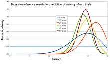
An archaeologist is working at a site thought to be from the medieval period, between the 11th century to the 16th century. However, it is uncertain exactly when in this period the site was inhabited. Fragments of pottery are found, some of which are glazed and some of which are decorated. It is expected that if the site were inhabited during the early medieval period, then 1% of the pottery would be glazed and 50% of its area decorated, whereas if it had been inhabited in the late medieval period then 81% would be glazed and 5% of its area decorated. How confident can the archaeologist be in the date of inhabitation as fragments are unearthed?

The degree of belief in the continuous variable $C$ (century) is to be calculated, with the discrete set of events $\{GD,G{\bar {D}},{\bar {G}}D,{\bar {G}}{\bar {D}}\}$ as evidence. Assuming linear variation of glaze and decoration with time, and that these variables are independent,

${\displaystyle P(E=GD\mid C=c)=(0.01+{\frac {0.81-0.01}{16-11}}(c-11))(0.5-{\frac {0.5-0.05}{16-11}}(c-11))}$

${\displaystyle P(E=G{\bar {D}}\mid C=c)=(0.01+{\frac {0.81-0.01}{16-11}}(c-11))(0.5+{\frac {0.5-0.05}{16-11}}(c-11))}$

${\displaystyle P(E={\bar {G}}D\mid C=c)=((1-0.01)-{\frac {0.81-0.01}{16-11}}(c-11))(0.5-{\frac {0.5-0.05}{16-11}}(c-11))}$

${\displaystyle P(E={\bar {G}}{\bar {D}}\mid C=c)=((1-0.01)-{\frac {0.81-0.01}{16-11}}(c-11))(0.5+{\frac {0.5-0.05}{16-11}}(c-11))}$

Assume a uniform prior of $\textstyle f_{C}(c)=0.2$, and that trials are independent and identically distributed. When a new fragment of type $e$ is discovered, Bayes' theorem is applied to update the degree of belief for each $c$:

$f_{C}(c\mid E=e)={\frac {P(E=e\mid C=c)}{P(E=e)}}f_{C}(c)={\frac {P(E=e\mid C=c)}{\int _{11}^{16}{P(E=e\mid C=c)f_{C}(c)dc}}}f_{C}(c)$

A computer simulation of the changing belief as 50 fragments are unearthed is shown on the graph. In the simulation, the site was inhabited around 1420, or $c=15.2$. By calculating the area under the relevant portion of the graph for 50 trials, the archaeologist can say that there is practically no chance the site was inhabited in the 11th and 12th centuries, about 1% chance that it was inhabited during the 13th century, 63% chance during the 14th century and 36% during the 15th century. Note that the Bernstein-von Mises theorem asserts here the asymptotic convergence to the "true" distribution because the probability space corresponding to the discrete set of events $\{GD,G{\bar {D}},{\bar {G}}D,{\bar {G}}{\bar {D}}\}$ is finite (see above section on asymptotic behaviour of the posterior).

In frequentist statistics and decision theory

A decision-theoretic justification of the use of Bayesian inference was given by Abraham Wald, who proved that every unique Bayesian procedure is admissible. Conversely, every admissible statistical procedure is either a Bayesian procedure or a limit of Bayesian procedures.^[7]

Wald characterized admissible procedures as Bayesian procedures (and limits of Bayesian procedures), making the Bayesian formalism a central technique in such areas of frequentist inference as parameter estimation, hypothesis testing, and computing confidence intervals.^[8] For example:

• "Under some conditions, all admissible procedures are either Bayes procedures or limits of Bayes procedures (in various senses). These remarkable results, at least in their original form, are due essentially to Wald. They are useful because the property of being Bayes is easier to analyze than admissibility."^[7]
• "In decision theory, a quite general method for proving admissibility consists in exhibiting a procedure as a unique Bayes solution."^[9]
• "In the first chapters of this work, prior distributions with finite support and the corresponding Bayes procedures were used to establish some of the main theorems relating to the comparison of experiments. Bayes procedures with respect to more general prior distributions have played a very important role in the development of statistics, including its asymptotic theory." "There are many problems where a glance at posterior distributions, for suitable priors, yields immediately interesting information. Also, this technique can hardly be avoided in sequential analysis."^[10]

• "A useful fact is that any Bayes decision rule obtained by taking a proper prior over the whole parameter space must be admissible"^[11]
• "An important area of investigation in the development of admissibility ideas has been that of conventional sampling-theory procedures, and many interesting results have been obtained."^[12]

Model selection

Applications

Computer applications

Bayesian inference has applications in artificial intelligence and expert systems. Bayesian inference techniques have been a fundamental part of computerized pattern recognition techniques since the late 1950s. There is also an ever growing connection between Bayesian methods and simulation-based Monte Carlo techniques since complex models cannot be processed in closed form by a Bayesian analysis, while a graphical model structure may allow for efficient simulation algorithms like the Gibbs sampling and other Metropolis–Hastings algorithm schemes.^[13] Recently Bayesian inference has gained popularity amongst the phylogenetics community for these reasons; a number of applications allow many demographic and evolutionary parameters to be estimated simultaneously.

As applied to statistical classification, Bayesian inference has been used in recent years to develop algorithms for identifying e-mail spam. Applications which make use of Bayesian inference for spam filtering include CRM114, DSPAM, Bogofilter, SpamAssassin, SpamBayes, Mozilla, XEAMS, and others. Spam classification is treated in more detail in the article on the naive Bayes classifier.

Solomonoff's Inductive inference is the theory of prediction based on observations; for example, predicting the next symbol based upon a given series of symbols. The only assumption is that the environment follows some unknown but computable probability distribution. It is a formal inductive framework that combines two well-studied principles of inductive inference: Bayesian statistics and Occam’s Razor.^[14] Solomonoff's universal prior probability of any prefix p of a computable sequence x is the sum of the probabilities of all programs (for a universal computer) that compute something starting with p. Given some p and any computable but unknown probability distribution from which x is sampled, the universal prior and Bayes' theorem can be used to predict the yet unseen parts of x in optimal fashion.^[15][16]

In the courtroom

Bayesian inference can be used by jurors to coherently accumulate the evidence for and against a defendant, and to see whether, in totality, it meets their personal threshold for 'beyond a reasonable doubt'.^[17][18][19] Bayes' theorem is applied successively to all evidence presented, with the posterior from one stage becoming the prior for the next. The benefit of a Bayesian approach is that it gives the juror an unbiased, rational mechanism for combining evidence. It may be appropriate to explain Bayes' theorem to jurors in odds form, as betting odds are more widely understood than probabilities. Alternatively, a logarithmic approach, replacing multiplication with addition, might be easier for a jury to handle.

Adding up evidence.

If the existence of the crime is not in doubt, only the identity of the culprit, it has been suggested that the prior should be uniform over the qualifying population.^[20] For example, if 1,000 people could have committed the crime, the prior probability of guilt would be 1/1000.

The use of Bayes' theorem by jurors is controversial. In the United Kingdom, a defence expert witness explained Bayes' theorem to the jury in R v Adams. The jury convicted, but the case went to appeal on the basis that no means of accumulating evidence had been provided for jurors who did not wish to use Bayes' theorem. The Court of Appeal upheld the conviction, but it also gave the opinion that "To introduce Bayes' Theorem, or any similar method, into a criminal trial plunges the jury into inappropriate and unnecessary realms of theory and complexity, deflecting them from their proper task."

Gardner-Medwin^[21] argues that the criterion on which a verdict in a criminal trial should be based is not the probability of guilt, but rather the probability of the evidence, given that the defendant is innocent (akin to a frequentist p-value). He argues that if the posterior probability of guilt is to be computed by Bayes' theorem, the prior probability of guilt must be known. This will depend on the incidence of the crime, which is an unusual piece of evidence to consider in a criminal trial. Consider the following three propositions:

A The known facts and testimony could have arisen if the defendant is guilty

B The known facts and testimony could have arisen if the defendant is innocent

C The defendant is guilty.

Gardner-Medwin argues that the jury should believe both A and not-B in order to convict. A and not-B implies the truth of C, but the reverse is not true. It is possible that B and C are both true, but in this case he argues that a jury should acquit, even though they know that they will be letting some guilty people go free. See also Lindley's paradox.

Bayesian epistemology

Bayesian epistemology is a movement that advocates for Bayesian inference as a means of justifying the rules of inductive logic.

Karl Popper and David Miller have rejected the alleged rationality of Bayesianism, i.e. using Bayes rule to make epistemological inferences:^[22] It is prone to the same vicious circle as any other justificationist epistemology, because it presupposes what it attempts to justify. According to this view, a rational interpretation of Bayesian inference would see it merely as a probabilistic version of falsification, rejecting the belief, commonly held by Bayesians, that high likelihood achieved by a series of Bayesian updates would prove the hypothesis beyond any reasonable doubt, or even with likelihood greater than 0.

Other

• The scientific method is sometimes interpreted as an application of Bayesian inference. In this view, Bayes' rule guides (or should guide) the updating of probabilities about hypotheses conditional on new observations or experiments.^[23]
• Bayesian search theory is used to search for lost objects.
• Bayesian inference in phylogeny
• Bayesian tool for methylation analysis
• Bayesian brain hypothesis says that the brain is a Bayesian mechanism.
• Bayesian inference in ecological studies^[24][25]

Bayes and Bayesian inference

The problem considered by Bayes in Proposition 9 of his essay, "An Essay towards solving a Problem in the Doctrine of Chances", is the posterior distribution for the parameter a (the success rate) of the binomial distribution.

History

The term Bayesian refers to Thomas Bayes (1702–1761), who proved a special case of what is now called Bayes' theorem. However, it was Pierre-Simon Laplace (1749–1827) who introduced a general version of the theorem and used it to approach problems in celestial mechanics, medical statistics, reliability, and jurisprudence.^[26] Early Bayesian inference, which used uniform priors following Laplace's principle of insufficient reason, was called "inverse probability" (because it infers backwards from observations to parameters, or from effects to causes^[27]). After the 1920s, "inverse probability" was largely supplanted by a collection of methods that came to be called frequentist statistics.^[27]

In the 20th century, the ideas of Laplace were further developed in two different directions, giving rise to objective and subjective currents in Bayesian practice. In the objective or "non-informative" current, the statistical analysis depends on only the model assumed, the data analyzed,^[28] and the method assigning the prior, which differs from one objective Bayesian to another objective Bayesian. In the subjective or "informative" current, the specification of the prior depends on the belief (that is, propositions on which the analysis is prepared to act), which can summarize information from experts, previous studies, etc.

In the 1980s, there was a dramatic growth in research and applications of Bayesian methods, mostly attributed to the discovery of Markov chain Monte Carlo methods, which removed many of the computational problems, and an increasing interest in nonstandard, complex applications.^[29] Despite growth of Bayesian research, most undergraduate teaching is still based on frequentist statistics.^[30] Nonetheless, Bayesian methods are widely accepted and used, such as for example in the field of machine learning.^[31]

See also

• Bayes' theorem
• Bayesian Analysis, the journal of the ISBA
• Bayesian hierarchical modeling
• Bayesian probability
• Inductive probability
• International Society for Bayesian Analysis (ISBA)
• Jeffreys prior
• Bayesian Structural Time Series (BSTS)
• Monty Hall problem

Notes

1. Hacking (1967, Section 3, p. 316), Hacking (1988, p. 124)
2. "Bayes' Theorem (Stanford Encyclopedia of Philosophy)". Plato.stanford.edu. Retrieved 2014-01-05.
3. van Fraassen, B. (1989) Laws and Symmetry, Oxford University Press. ISBN 0-19-824860-1
4. Gelman, Andrew; Carlin, John B.; Stern, Hal S.; Dunson, David B.;Vehtari, Aki; Rubin, Donald B. (2013). Bayesian Data Analysis, Third Edition. Chapman and Hall/CRC. ISBN 978-1-4398-4095-5.
5. Larry Wasserman et alia, JASA 2000.
6. Sen, Pranab K.; Keating, J. P.; Mason, R. L. (1993). Pitman's measure of closeness: A comparison of statistical estimators. Philadelphia: SIAM.
7. Bickel & Doksum (2001, p. 32)
8. • Kiefer, J.; Schwartz R. (1965). "Admissible Bayes Character of T²-, R²-, and Other Fully Invariant Tests for Multivariate Normal Problems". Annals of Mathematical Statistics. 36: 747–770. doi:10.1214/aoms/1177700051.
   • Schwartz, R. (1969). "Invariant Proper Bayes Tests for Exponential Families". Annals of Mathematical Statistics. 40: 270–283. doi:10.1214/aoms/1177697822.
   • Hwang, J. T. & Casella, George (1982). "Minimax Confidence Sets for the Mean of a Multivariate Normal Distribution". Annals of Statistics. 10: 868–881. doi:10.1214/aos/1176345877.
9. Lehmann, Erich (1986). Testing Statistical Hypotheses (Second ed.). (see p. 309 of Chapter 6.7 "Admissibilty", and pp. 17–18 of Chapter 1.8 "Complete Classes"
10. Le Cam, Lucien (1986). Asymptotic Methods in Statistical Decision Theory. Springer-Verlag. ISBN 0-387-96307-3. (From "Chapter 12 Posterior Distributions and Bayes Solutions", p. 324)
11. Cox, D. R.; Hinkley, D.V (1974). Theoretical Statistics. Chapman and Hall. ISBN 0-04-121537-0. page 432
12. Cox, D. R.; Hinkley, D. V. (1974). Theoretical Statistics. Chapman and Hall. ISBN 0-04-121537-0. p. 433)
13. Jim Albert (2009). Bayesian Computation with R, Second edition. New York, Dordrecht, etc.: Springer. ISBN 978-0-387-92297-3.
14. Samuel Rathmanner and Marcus Hutter. "A Philosophical Treatise of Universal Induction". Entropy, 13(6):1076–1136, 2011.
15. "The Problem of Old Evidence", in §5 of "On Universal Prediction and Bayesian Confirmation", M. Hutter - Theoretical Computer Science, 2007 - Elsevier
16. "Raymond J. Solomonoff", Peter Gacs, Paul M. B. Vitanyi, 2011 cs.bu.edu
17. Dawid, A. P. and Mortera, J. (1996) "Coherent Analysis of Forensic Identification Evidence". Journal of the Royal Statistical Society, Series B, 58, 425–443.
18. Foreman, L. A.; Smith, A. F. M., and Evett, I. W. (1997). "Bayesian analysis of deoxyribonucleic acid profiling data in forensic identification applications (with discussion)". Journal of the Royal Statistical Society, Series A, 160, 429–469.
19. Robertson, B. and Vignaux, G. A. (1995) Interpreting Evidence: Evaluating Forensic Science in the Courtroom. John Wiley and Sons. Chichester. ISBN 978-0-471-96026-3
20. Dawid, A. P. (2001) Bayes' Theorem and Weighing Evidence by Juries
21. Gardner-Medwin, A. (2005) "What Probability Should the Jury Address?". Significance, 2 (1), March 2005
22. David Miller: Critical Rationalism
23. Howson & Urbach (2005), Jaynes (2003)
24. Ogle, Kiona; Tucker, Colin; Cable, Jessica M. (2014-01-01). "Beyond simple linear mixing models: process-based isotope partitioning of ecological processes". Ecological Applications. 24 (1): 181–195. doi:10.1890/1051-0761-24.1.181. ISSN 1939-5582.
25. Evaristo, Jaivime; McDonnell, Jeffrey J.; Scholl, Martha A.; Bruijnzeel, L. Adrian; Chun, Kwok P. (2016-01-01). "Insights into plant water uptake from xylem-water isotope measurements in two tropical catchments with contrasting moisture conditions". Hydrological Processes: n/a–n/a. doi:10.1002/hyp.10841. ISSN 1099-1085.
26. Stigler, Stephen M. (1986). "Chapter 3". The History of Statistics. Harvard University Press.
27. Fienberg, Stephen E. (2006). "When did Bayesian Inference Become 'Bayesian'?" (PDF). Bayesian Analysis. 1 (1): 1–40 [p. 5]. doi:10.1214/06-ba101. Archived from the original (PDF) on 2014-09-10.
28. Bernardo, José-Miguel (2005). "Reference analysis". Handbook of statistics. 25. pp. 17–90.
29. Wolpert, R. L. (2004). "A Conversation with James O. Berger". Statistical Science. 19 (1): 205–218. doi:10.1214/088342304000000053. MR 2082155.
30. Bernardo, José M. (2006). "A Bayesian mathematical statistics primer" (PDF). ICOTS-7.
31. Bishop, C. M. (2007). Pattern Recognition and Machine Learning. New York: Springer. ISBN 0387310738.

References

• Aster, Richard; Borchers, Brian, and Thurber, Clifford (2012). Parameter Estimation and Inverse Problems, Second Edition, Elsevier. ISBN 0123850487, ISBN 978-0123850485
• Bickel, Peter J. & Doksum, Kjell A. (2001). Mathematical Statistics, Volume 1: Basic and Selected Topics (Second (updated printing 2007) ed.). Pearson Prentice–Hall. ISBN 0-13-850363-X.
• Box, G. E. P. and Tiao, G. C. (1973) Bayesian Inference in Statistical Analysis, Wiley, ISBN 0-471-57428-7
• Edwards, Ward (1968). "Conservatism in Human Information Processing". In Kleinmuntz, B. Formal Representation of Human Judgment. Wiley.
• Edwards, Ward (1982). "Conservatism in Human Information Processing (excerpted)". In Daniel Kahneman, Paul Slovic and Amos Tversky. Judgment under uncertainty: Heuristics and biases. Cambridge University Press.
• Jaynes E. T. (2003) Probability Theory: The Logic of Science, CUP. ISBN 978-0-521-59271-0 (Link to Fragmentary Edition of March 1996).
• Howson, C. & Urbach, P. (2005). Scientific Reasoning: the Bayesian Approach (3rd ed.). Open Court Publishing Company. ISBN 978-0-8126-9578-6.
• Phillips, L. D.; Edwards, Ward (October 2008). "Chapter 6: Conservatism in a Simple Probability Inference Task (Journal of Experimental Psychology (1966) 72: 346-354)". In Jie W. Weiss; David J. Weiss. A Science of Decision Making:The Legacy of Ward Edwards. Oxford University Press. p. 536. ISBN 978-0-19-532298-9.

Further reading

• For a full report on the history of Bayesian statistics and the debates with frequentists approaches, read Vallverdu, Jordi (2016). Bayesians Versus Frequentists A Philosophical Debate on Statistical Reasoning. New York: Springer. ISBN 978-3-662-48638-2.

Elementary

The following books are listed in ascending order of probabilistic sophistication:

• Stone, JV (2013), "Bayes’ Rule: A Tutorial Introduction to Bayesian Analysis", Download first chapter here, Sebtel Press, England.
• Dennis V. Lindley (2013). Understanding Uncertainty, Revised Edition (2nd ed.). John Wiley. ISBN 978-1-118-65012-7.
• Colin Howson & Peter Urbach (2005). Scientific Reasoning: The Bayesian Approach (3rd ed.). Open Court Publishing Company. ISBN 978-0-8126-9578-6.
• Berry, Donald A. (1996). Statistics: A Bayesian Perspective. Duxbury. ISBN 0-534-23476-3.
• Morris H. DeGroot & Mark J. Schervish (2002). Probability and Statistics (third ed.). Addison-Wesley. ISBN 978-0-201-52488-8.
• Bolstad, William M. (2007) Introduction to Bayesian Statistics: Second Edition, John Wiley ISBN 0-471-27020-2
• Winkler, Robert L (2003). Introduction to Bayesian Inference and Decision (2nd ed.). Probabilistic. ISBN 0-9647938-4-9. Updated classic textbook. Bayesian theory clearly presented.
• Lee, Peter M. Bayesian Statistics: An Introduction. Fourth Edition (2012), John Wiley ISBN 978-1-1183-3257-3
• Carlin, Bradley P. & Louis, Thomas A. (2008). Bayesian Methods for Data Analysis, Third Edition. Boca Raton, FL: Chapman and Hall/CRC. ISBN 1-58488-697-8.
• Gelman, Andrew; Carlin, John B.; Stern, Hal S.; Dunson, David B.; Vehtari, Aki; Rubin, Donald B. (2013). Bayesian Data Analysis, Third Edition. Chapman and Hall/CRC. ISBN 978-1-4398-4095-5.

Intermediate or advanced

• Berger, James O (1985). Statistical Decision Theory and Bayesian Analysis. Springer Series in Statistics (Second ed.). Springer-Verlag. ISBN 0-387-96098-8.
• Bernardo, José M.; Smith, Adrian F. M. (1994). Bayesian Theory. Wiley.
• DeGroot, Morris H., Optimal Statistical Decisions. Wiley Classics Library. 2004. (Originally published (1970) by McGraw-Hill.) ISBN 0-471-68029-X.
• Schervish, Mark J. (1995). Theory of statistics. Springer-Verlag. ISBN 0-387-94546-6.
• Jaynes, E. T. (1998) Probability Theory: The Logic of Science.
• O'Hagan, A. and Forster, J. (2003) Kendall's Advanced Theory of Statistics, Volume 2B: Bayesian Inference. Arnold, New York. ISBN 0-340-52922-9.
• Robert, Christian P (2001). The Bayesian Choice – A Decision-Theoretic Motivation (second ed.). Springer. ISBN 0-387-94296-3.
• Glenn Shafer and Pearl, Judea, eds. (1988) Probabilistic Reasoning in Intelligent Systems, San Mateo, CA: Morgan Kaufmann.
• Pierre Bessière et al. (2013), "Bayesian Programming", CRC Press. ISBN 9781439880326
• Francisco J. Samaniego (2010), "A Comparison of the Bayesian and Frequentist Approaches to Estimation" Springer, New York, ISBN 978-1-4419-5940-9

External links

• Hazewinkel, Michiel, ed. (2001), "Bayesian approach to statistical problems", Encyclopedia of Mathematics, Springer, ISBN 978-1-55608-010-4
• Bayesian Statistics from Scholarpedia.
• Introduction to Bayesian probability from Queen Mary University of London
• Mathematical Notes on Bayesian Statistics and Markov Chain Monte Carlo
• Bayesian reading list, categorized and annotated by Tom Griffiths
• A. Hajek and S. Hartmann: Bayesian Epistemology, in: J. Dancy et al. (eds.), A Companion to Epistemology. Oxford: Blackwell 2010, 93-106.
• S. Hartmann and J. Sprenger: Bayesian Epistemology, in: S. Bernecker and D. Pritchard (eds.), Routledge Companion to Epistemology. London: Routledge 2010, 609-620.
• Stanford Encyclopedia of Philosophy: "Inductive Logic"
• Bayesian Confirmation Theory
• What Is Bayesian Learning?