Coxeter–Dynkin diagram


In geometry, a Coxeter–Dynkin diagram (or Coxeter diagram, Coxeter graph) is a graph with numerically labeled edges (called branches) representing the spatial relations between a collection of mirrors (or reflecting hyperplanes). It describes a kaleidoscopic construction: each graph "node" represents a mirror (domain facet) and the label attached to a branch encodes the dihedral angle order between two mirrors (on a domain ridge). An unlabeled branch implicitly represents order-3.
Each diagram represents a Coxeter group, and Coxeter groups are classified by their associated diagrams.
Dynkin diagrams are closely related objects, which differ from Coxeter diagrams in two respects: firstly, branches labeled "4" or greater are directed, while Coxeter diagrams are undirected; secondly, Dynkin diagrams must satisfy an additional (crystallographic) restriction, namely that the only allowed branch labels are 2, 3, 4, and 6. Dynkin diagrams correspond to and are used to classify root systems and therefore semisimple Lie algebras.[1]
Description
Branches of a Coxeter–Dynkin diagram are labeled with a rational number p, representing a dihedral angle of 180°/p. When p = 2 the angle is 90° and the mirrors have no interaction, so the branch can be omitted from the diagram. If a branch is unlabeled, it is assumed to have p = 3, representing an angle of 60°. Two parallel mirrors have a branch marked with "∞". In principle, n mirrors can be represented by a complete graph in which all n(n − 1) / 2 branches are drawn. In practice, nearly all interesting configurations of mirrors include a number of right angles, so the corresponding branches are omitted.
Diagrams can be labeled by their graph structure. The first forms studied by Ludwig Schläfli are the orthoschemes which have linear graphs that generate regular polytopes and regular honeycombs. Plagioschemes are simplices represented by branching graphs, and cycloschemes are simplices represented by cyclic graphs.
Schläfli matrix
Every Coxeter diagram has a corresponding Schläfli matrix with matrix elements ai,j = aj,i = −2cos (π / p) where p is the branch order between the pairs of mirrors. As a matrix of cosines, it is also called a Gramian matrix after Jørgen Pedersen Gram. All Coxeter group Schläfli matrices are symmetric because their root vectors are normalized. It is related closely to the Cartan matrix, used in the similar but directed graph Dynkin diagrams in the limited cases of p = 2,3,4, and 6, which are NOT symmetric in general.
The determinant of the Schläfli matrix, called the Schläflian, and its sign determines whether the group is finite (positive), affine (zero), indefinite (negative). This rule is called Schläfli's Criterion.[2]
The eigenvalues of the Schläfli matrix determines whether a Coxeter group is of finite type (all positive), affine type (all non-negative, at least one is zero), or indefinite type (otherwise). The indefinite type is sometimes further subdivided, e.g. into hyperbolic and other Coxeter groups. However, there are multiple non-equivalent definitions for hyperbolic Coxeter groups. We use the following definition: A Coxeter group with connected diagram is hyperbolic if it is neither of finite nor affine type, but every proper connected subdiagram is of finite or affine type. A hyperbolic Coxeter group is compact if all subgroups are finite (i.e. have positive determinants), and paracompact if all its subgroups are finite or affine (i.e. have nonnegative determinants).
Finite and affine groups are also called elliptical and parabolic respectively. Hyperbolic groups are also called Lannér, after F. Lannér who enumerated the compact hyperbolic groups in 1950,[3] and Koszul (or quasi-Lannér) for the paracompact groups.
Rank 2 Coxeter groups
For rank 2, the type of a Coxeter group is fully determined by the determinant of the Schläfli matrix, as it is simply the product of the eigenvalues: Finite type (positive determinant), affine type (zero determinant) or hyperbolic (negative determinant). Coxeter uses an equivalent bracket notation which lists sequences of branch orders as a substitute for the node-branch graphic diagrams. Rational solutions [p/q], ![]()
![]()
![]()
![]()
![]() , also exist, with gcd(p,q)=1, which define overlapping fundamental domains. For example, 3/2, 4/3, 5/2, 5/3, 5/4. and 6/5.
, also exist, with gcd(p,q)=1, which define overlapping fundamental domains. For example, 3/2, 4/3, 5/2, 5/3, 5/4. and 6/5.
| Type | Finite | Affine | Hyperbolic | |||||
|---|---|---|---|---|---|---|---|---|
| Geometry |  |
 |
 |
 |
... |  |
 |
 |
| Coxeter | [ ] |
[2] |
[3] |
[4] |
[p] |
[∞] |
[∞] |
[iπ/λ] |
| Order | 2 | 4 | 6 | 8 | 2p | ∞ | ||
| Mirror lines are colored to correspond to Coxeter diagram nodes. Fundamental domains are alternately colored. | ||||||||
| Order p |
Group | Coxeter diagram | Schläfli matrix | |||
|---|---|---|---|---|---|---|
| Determinant (4-a21*a12) | ||||||
| Finite (Determinant>0) | ||||||
| 2 | I2(2) = A1xA1 | [2] | 4 | |||
| 3 | I2(3) = A2 | [3] | 3 | |||
| 3/2 | [3/2] | |||||
| 4 | I2(4) = B2 | [4] | 2 | |||
| 4/3 | [4/3] | |||||
| 5 | I2(5) = H2 | [5] | ~1.38196601125 | |||
| 5/4 | [5/4] | |||||
| 5/2 | [5/2] | ~3.61803398875 | ||||
| 5/3 | [5/3] | |||||
| 6 | I2(6) = G2 | [6] | 1 | |||
| 6/5 | [6/5] | |||||
| 8 | I2(8) | [8] | ~0.58578643763 | |||
| 10 | I2(10) | [10] | = ~0.38196601125 | |||
| 12 | I2(12) | [12] | ~0.26794919243 | |||
| p | I2(p) | [p] | ||||
| Affine (Determinant=0) | ||||||
| ∞ | I2(∞) = = | [∞] | 0 | |||
| Hyperbolic (Determinant≤0) | ||||||
| ∞ | [∞] | 0 | ||||
| ∞ | [iπ/λ] | |||||
![\left[{\begin{matrix}2&a_{12}\\a_{21}&2\end{matrix}}\right]](../I/m/609b9b4324da49c4903330c430b14203d6f971cb.svg)
![\left[{\begin{smallmatrix}2&0\\0&2\end{smallmatrix}}\right]](../I/m/58d402f7fd38428fe2ac791f5a5d12bf7832c69f.svg)
![\left[{\begin{smallmatrix}2&-1\\-1&2\end{smallmatrix}}\right]](../I/m/18cb26b504d63dba11f3a12c7ee8fa25fe3bdf0a.svg)
![{\displaystyle \left[{\begin{smallmatrix}2&1\\1&2\end{smallmatrix}}\right]}](../I/m/838a30dc9d065ec434dff490bd84061ed569db3b.svg)
![\left[{\begin{smallmatrix}2&-{\sqrt {2}}\\-{\sqrt {2}}&2\end{smallmatrix}}\right]](../I/m/934421fb85592c1788a92b7d350953dd2ca94b5e.svg)
![{\displaystyle \left[{\begin{smallmatrix}2&{\sqrt {2}}\\{\sqrt {2}}&2\end{smallmatrix}}\right]}](../I/m/4f92222bfe2eeefe46dddcc56620241d8efd5ef1.svg)
![\left[{\begin{smallmatrix}2&-\phi \\-\phi &2\end{smallmatrix}}\right]](../I/m/db286eb5ca733d2b6ab1c5f194f03593440b5b3a.svg)

![{\displaystyle \left[{\begin{smallmatrix}2&\phi \\\phi &2\end{smallmatrix}}\right]}](../I/m/3dcf61f3b1fac33acafec6ac2d577c66f9f69306.svg)
![{\displaystyle \left[{\begin{smallmatrix}2&1-\phi \\1-\phi &2\end{smallmatrix}}\right]}](../I/m/4a16582176db9cb488aa850d0b0a970ff0a62cd6.svg)

![{\displaystyle \left[{\begin{smallmatrix}2&\phi -1\\\phi -1&2\end{smallmatrix}}\right]}](../I/m/8548776ee20b1e4a17df57227d372025e5bcbd65.svg)
![\left[{\begin{smallmatrix}2&-{\sqrt {3}}\\-{\sqrt {3}}&2\end{smallmatrix}}\right]](../I/m/3b77e92921199a57f051014d4938de1a0d22ef38.svg)
![{\displaystyle \left[{\begin{smallmatrix}2&{\sqrt {3}}\\{\sqrt {3}}&2\end{smallmatrix}}\right]}](../I/m/51483cac6134b485a8a8ea0d9e2fee62fda6d13a.svg)
![\left[{\begin{smallmatrix}2&-2\cos(\pi /8)\\-2\cos(\pi /8)&2\end{smallmatrix}}\right]](../I/m/aa253a5d705d6109194b3afc3fe1d07614f51096.svg)

![\left[{\begin{smallmatrix}2&-2\cos(\pi /10)\\-2\cos(\pi /10)&2\end{smallmatrix}}\right]](../I/m/c3bd41acbb86ee3d9cdaf3b56cd15f8dd58b4766.svg)


![\left[{\begin{smallmatrix}2&-2\cos(\pi /12)\\-2\cos(\pi /12)&2\end{smallmatrix}}\right]](../I/m/2169b8ecb32a8780141f79c1340adff5c4eea986.svg)

![\left[{\begin{smallmatrix}2&-2\cos(\pi /p)\\-2\cos(\pi /p)&2\end{smallmatrix}}\right]](../I/m/71dd5a3c2a3aa08ab89d00e05a0afe4db4876ff8.svg)


![\left[{\begin{smallmatrix}2&-2\\-2&2\end{smallmatrix}}\right]](../I/m/cd86323eaf497d2bb96f757556dd458abd5863cf.svg)
![\left[{\begin{smallmatrix}2&-2cosh(2\lambda )\\-2cosh(2\lambda )&2\end{smallmatrix}}\right]](../I/m/274a1c42213fa3aad2dd64c4b63f424d5f3ed349.svg)

Geometric visualizations
The Coxeter–Dynkin diagram can be seen as a graphic description of the fundamental domain of mirrors. A mirror represents a hyperplane within a given dimensional spherical or Euclidean or hyperbolic space. (In 2D spaces, a mirror is a line, and in 3D a mirror is a plane).
These visualizations show the fundamental domains for 2D and 3D Euclidean groups, and 2D spherical groups. For each the Coxeter diagram can be deduced by identifying the hyperplane mirrors and labelling their connectivity, ignoring 90-degree dihedral angles (order 2).
 Coxeter groups in the Euclidean plane with equivalent diagrams. Reflections are labeled as graph nodes R1, R2, etc. and are colored by their reflection order. Reflections at 90 degrees are inactive and therefore suppressed from the diagram. Parallel mirrors are connected by an ∞ labeled branch. The prismatic group x is shown as a doubling of the , but can also be created as rectangular domains from doubling the triangles. The is a doubling of the triangle. | |
 Many Coxeter groups in the hyperbolic plane can be extended from the Euclidean cases as a series of hyperbolic solutions. | |
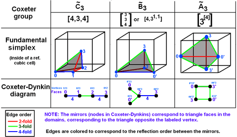 Coxeter groups in 3-space with diagrams. Mirrors (triangle faces) are labeled by opposite vertex 0..3. Branches are colored by their reflection order. fills 1/48 of the cube. fills 1/24 of the cube. fills 1/12 of the cube. |
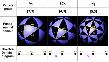 Coxeter groups in the sphere with equivalent diagrams. One fundamental domain is outlined in yellow. Domain vertices (and graph branches) are colored by their reflection order. |


Finite Coxeter groups
- See also polytope families for a table of end-node uniform polytopes associated with these groups.
- Three different symbols are given for the same groups – as a letter/number, as a bracketed set of numbers, and as the Coxeter diagram.
- The bifurcated Dn groups is half or alternated version of the regular Cn groups.
- The bifurcated Dn and En groups are also labeled by a superscript form [3a,b,c] where a,b,c are the numbers of segments in each of the three branches.
| Rank | Simple Lie groups | Exceptional Lie groups | ||||||
|---|---|---|---|---|---|---|---|---|
| 1 | A1=[ ] |
|||||||
| 2 | A2=[3] |
B2=[4] |
D2=A1A1 |
G2=[6] |
H2=[5] |
I2[p] | ||
| 3 | A3=[32] |
B3=[3,4] |
D3=A3 |
E3=A2A1 |
F3=B3 |
H3 |
||
| 4 | A4=[33] |
B4=[32,4] |
D4=[31,1,1] |
E4=A4 |
F4 |
H4 | ||
| 5 | A5=[34] |
B5=[33,4] |
D5=[32,1,1] |
E5=D5 |
||||
| 6 | A6=[35] |
B6=[34,4] |
D6=[33,1,1] |
E6=[32,2,1] | ||||
| 7 | A7=[36] |
B7=[35,4] |
D7=[34,1,1] |
E7=[33,2,1] | ||||
| 8 | A8=[37] |
B8=[36,4] |
D8=[35,1,1] |
E8=[34,2,1] | ||||
| 9 | A9=[38] |
B9=[37,4] |
D9=[36,1,1] |
|||||
| 10+ | .. | .. | .. | .. | ||||


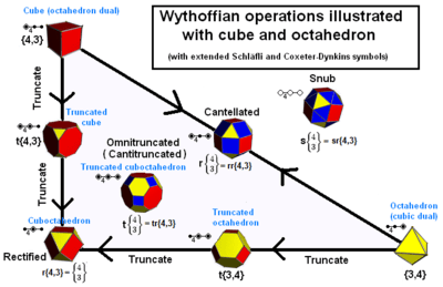
Application with uniform polytopes

Coxeter–Dynkin diagrams can explicitly enumerate nearly all classes of uniform polytope and uniform tessellations. Every uniform polytope with pure reflective symmetry (all but a few special cases have pure reflectional symmetry) can be represented by a Coxeter–Dynkin diagram with permutations of markups. Each uniform polytope can be generated using such mirrors and a single generator point: mirror images create new points as reflections, then polytope edges can be defined between points and a mirror image point. Faces can be constructed by cycles of edges created, etc. To specify the generating vertex, one or more nodes are marked with rings, meaning that the vertex is not on the mirror(s) represented by the ringed node(s). (If two or more mirrors are marked, the vertex is equidistant from them.) A mirror is active (creates reflections) only with respect to points not on it. A diagram needs at least one active node to represent a polytope.
All regular polytopes, represented by Schläfli symbol {p, q, r, ...}, can have their fundamental domains represented by a set of n mirrors with a related Coxeter–Dynkin diagram of a line of nodes and branches labeled by p, q, r, ..., with the first node ringed.
Uniform polytopes with one ring correspond to generator points at the corners of the fundamental domain simplex. Two rings correspond to the edges of simplex and have a degree of freedom, with only the midpoint as the uniform solution for equal edge lengths. In general k-ring generator points are on (k-1)-faces of the simplex, and if all the nodes are ringed, the generator point is in the interior of the simplex.
A secondary markup conveys a special case nonreflectional symmetry uniform polytopes. These cases exist as alternations of reflective symmetry polytopes. This markup removes the central dot of a ringed node, called a hole (circles with nodes removed), to imply alternate nodes deleted. The resulting polytope will have a subsymmetry of the original Coxeter group. A truncated alternation is called a snub.
- A single node represents a single mirror. This is called group A1. If ringed this creates a line segment perpendicular to the mirror, represented as {}.
- Two unattached nodes represent two perpendicular mirrors. If both nodes are ringed, a rectangle can be created, or a square if the point is at equal distance from both mirrors.
- Two nodes attached by an order-n branch can create an n-gon if the point is on one mirror, and a 2n-gon if the point is off both mirrors. This forms the I1(n) group.
- Two parallel mirrors can represent an infinite polygon I1(∞) group, also called Ĩ1.
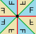
- Three mirrors in a triangle form images seen in a traditional kaleidoscope and can be represented by three nodes connected in a triangle. Repeating examples will have branches labeled as (3 3 3), (2 4 4), (2 3 6), although the last two can be drawn as a line (with the 2 branches ignored). These will generate uniform tilings.
- Three mirrors can generate uniform polyhedra; including rational numbers gives the set of Schwarz triangles.
- Three mirrors with one perpendicular to the other two can form the uniform prisms.
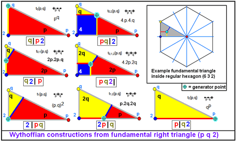 There are 7 reflective uniform constructions within a general triangle, based on 7 topological generator positions within the fundamental domain. Every active mirror generates an edge, with two active mirrors have generators on the domain sides and three active mirrors has the generator in the interior. One or two degrees of freedom can be solved for a unique position for equal edge lengths of the resulting polyhedron or tiling. |
 Example 7 generators on octahedral symmetry, fundamental domain triangle (4 3 2), with 8th snub generation as an alternation |
The duals of the uniform polytopes are sometimes marked up with a perpendicular slash replacing ringed nodes, and a slash-hole for hole nodes of the snubs. For example, ![]()
![]()
![]() represents a rectangle (as two active orthogonal mirrors), and
represents a rectangle (as two active orthogonal mirrors), and ![]()
![]()
![]() represents its dual polygon, the rhombus.
represents its dual polygon, the rhombus.
Example polyhedra and tilings
For example, the B3 Coxeter group has a diagram: ![]()
![]()
![]()
![]()
![]() . This is also called octahedral symmetry.
. This is also called octahedral symmetry.
There are 7 convex uniform polyhedra that can be constructed from this symmetry group and 3 from its alternation subsymmetries, each with a uniquely marked up Coxeter–Dynkin diagram. The Wythoff symbol represents a special case of the Coxeter diagram for rank 3 graphs, with all 3 branch orders named, rather than suppressing the order 2 branches. The Wythoff symbol is able to handle the snub form, but not general alternations without all nodes ringed.
| Uniform octahedral polyhedra | ||||||||||
|---|---|---|---|---|---|---|---|---|---|---|
| Symmetry: [4,3], (*432) | [4,3]+ (432) |
[1+,4,3] = [3,3] (*332) |
[3+,4] (3*2) | |||||||
| {4,3} | t{4,3} | r{4,3} r{31,1} |
t{3,4} t{31,1} |
{3,4} {31,1} |
rr{4,3} s2{3,4} |
tr{4,3} | sr{4,3} | h{4,3} {3,3} |
h2{4,3} t{3,3} |
s{3,4} s{31,1} |
= |
= |
= |
||||||||
| Duals to uniform polyhedra | ||||||||||
| V43 | V3.82 | V(3.4)2 | V4.62 | V34 | V3.43 | V4.6.8 | V34.4 | V33 | V3.62 | V35 |
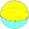
The same constructions can be made on disjointed (orthogonal) Coxeter groups like the uniform prisms, and can be seen more clearly as tilings of dihedrons and hosohedrons on the sphere, like this [6]×[] or [6,2] family:
| Uniform hexagonal dihedral spherical polyhedra | ||||||||||||||
|---|---|---|---|---|---|---|---|---|---|---|---|---|---|---|
| Symmetry: [6,2], (*622) | [6,2]+, (622) | [6,2+], (2*3) | ||||||||||||
 |
|
|
 |
 |
|
 |
 |
 | ||||||
| {6,2} | t{6,2} | r{6,2} | t{2,6} | {2,6} | rr{6,2} | tr{6,2} | sr{6,2} | s{2,6} | ||||||
| Duals to uniforms | ||||||||||||||
| |
 |
|
 |
|
|
 |
 |
 | ||||||
| V62 | V122 | V62 | V4.4.6 | V26 | V4.4.6 | V4.4.12 | V3.3.3.6 | V3.3.3.3 | ||||||
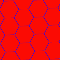
In comparison, the [6,3], ![]()
![]()
![]()
![]()
![]() family produces a parallel set of 7 uniform tilings of the Euclidean plane, and their dual tilings. There are again 3 alternations and some half symmetry version.
family produces a parallel set of 7 uniform tilings of the Euclidean plane, and their dual tilings. There are again 3 alternations and some half symmetry version.
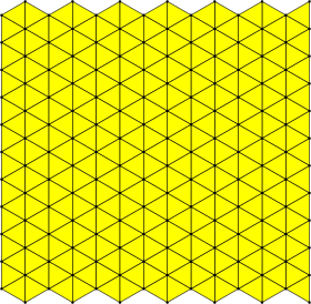
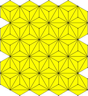
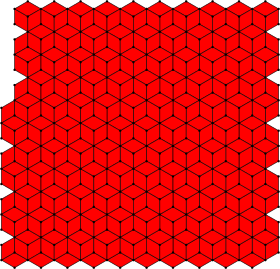
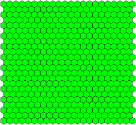
| Uniform hexagonal/triangular tilings | |||||||||||
|---|---|---|---|---|---|---|---|---|---|---|---|
| Symmetry: [6,3], (*632) | [6,3]+ (632) |
[6,3+] (3*3) | |||||||||
| {6,3} | t{6,3} | r{6,3} | t{3,6} | {3,6} | rr{6,3} | tr{6,3} | sr{6,3} | s{3,6} | |||
 |
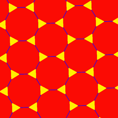 |
 |
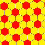 |
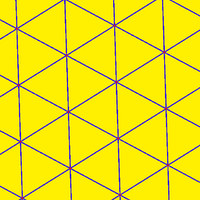 |
 |
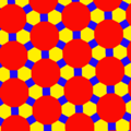 |
 |
 | |||
| 63 | 3.122 | (3.6)2 | 6.6.6 | 36 | 3.4.12.4 | 4.6.12 | 3.3.3.3.6 | 3.3.3.3.3.3 | |||
| Uniform duals | |||||||||||
 |
 |
 |
 |
|
 |
 |
 |
| |||
| V63 | V3.122 | V(3.6)2 | V63 | V36 | V3.4.12.4 | V.4.6.12 | V34.6 | V36 | |||
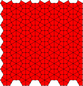
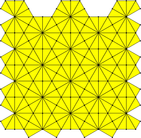
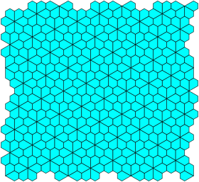
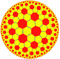
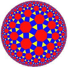
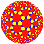
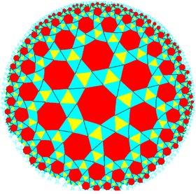
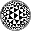
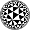
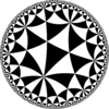
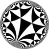
In the hyperbolic plane [7,3], ![]()
![]()
![]()
![]()
![]() family produces a parallel set of uniform tilings of the Euclidean plane, and their dual tilings. There is only 1 alternation (snub) since all branch orders are odd. Many other hyperbolic families of uniform tilings can be seen at uniform tilings in hyperbolic plane.
family produces a parallel set of uniform tilings of the Euclidean plane, and their dual tilings. There is only 1 alternation (snub) since all branch orders are odd. Many other hyperbolic families of uniform tilings can be seen at uniform tilings in hyperbolic plane.
| Uniform heptagonal/triangular tilings | |||||||||||
|---|---|---|---|---|---|---|---|---|---|---|---|
| Symmetry: [7,3], (*732) | [7,3]+, (732) | ||||||||||
 |
 |
 |
 |
 |
 |
 |
 | ||||
| {7,3} | t{7,3} | r{7,3} | t{3,7} | {3,7} | rr{7,3} | tr{7,3} | sr{7,3} | ||||
| Uniform duals | |||||||||||
|
 |
 |
 |
|
 |
 |
 | ||||
| V73 | V3.14.14 | V3.7.3.7 | V6.6.7 | V37 | V3.4.7.4 | V4.6.14 | V3.3.3.3.7 | ||||
Affine Coxeter groups
Families of convex uniform Euclidean tessellations are defined by the affine Coxeter groups. These groups are identical to the finite groups with the inclusion of one added node. In letter names they are given the same letter with a "~" above the letter. The index refers to the finite group, so the rank is the index plus 1. (Ernst Witt symbols for the affine groups are given as also)
- : diagrams of this type are cycles. (Also Pn)
- is associated with the hypercube regular tessellation {4, 3, ...., 4} family. (Also Rn)
- related to C by one removed mirror. (Also Sn)
- related to C by two removed mirrors. (Also Qn)
- , , . (Also T7, T8, T9)
- forms the {3,4,3,3} regular tessellation. (Also U5)
- forms 30-60-90 triangle fundamental domains. (Also V3)
- is two parallel mirrors. ( = = ) (Also W2)


Composite groups can also be defined as orthogonal projects. The most common use , like , ![]()
![]()
![]()
![]()
![]()
![]()
![]() represents square or rectangular checker board domains in the Euclidean plane. And
represents square or rectangular checker board domains in the Euclidean plane. And ![]()
![]()
![]()
![]()
![]()
![]()
![]() represents triangular prism fundamental domains in Euclidean 3-space.
represents triangular prism fundamental domains in Euclidean 3-space.


| Rank | (P2+) | (S4+) | (R2+) | (Q5+) | (Tn+1) / (U5) / (V3) |
|---|---|---|---|---|---|
| 2 | =[∞] |
=[∞] |
|||
| 3 | =[3[3]] * |
=[4,4] * |
=[6,3] * | ||
| 4 | =[3[4]] * |
=[4,31,1] * |
=[4,3,4] * |
=[31,1,3−1,31,1] |
|
| 5 | =[3[5]] * |
=[4,3,31,1] * |
=[4,32,4] * |
=[31,1,1,1] * |
=[3,4,3,3] * |
| 6 | =[3[6]] * |
=[4,32,31,1] * |
=[4,33,4] * |
=[31,1,3,31,1] * |
|
| 7 | =[3[7]] * |
=[4,33,31,1] |
=[4,34,4] |
=[31,1,32,31,1] |
=[32,2,2] |
| 8 | =[3[8]] * |
=[4,34,31,1] * |
=[4,35,4] |
=[31,1,33,31,1] * |
=[33,3,1] * |
| 9 | =[3[9]] * |
=[4,35,31,1] |
=[4,36,4] |
=[31,1,34,31,1] |
=[35,2,1] * |
| 10 | =[3[10]] * |
=[4,36,31,1] |
=[4,37,4] |
=[31,1,35,31,1] | |
| 11 | ... | ... | ... | ... |


Hyperbolic Coxeter groups
There are many infinite hyperbolic Coxeter groups. Hyperbolic groups are categorized as compact or not, with compact groups having bounded fundamental domains. Compact simplex hyperbolic groups (Lannér simplices) exist as rank 3 to 5. Paracompact simplex groups (Koszul simplices) exist up to rank 10. Hypercompact (Vinberg polytopes) groups have been explored but not been fully determined. In 2006, Allcock proved that there are infinitely many compact Vinberg polytopes for dimension up to 6, and infinitely many finite-volume Vinberg polytopes for dimension up to 19,[4] so a complete enumeration is not possible. All of these fundamental reflective domains, both simplices and nonsimplices, are often called Coxeter polytopes or sometimes less accurately Coxeter polyhedra.
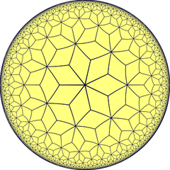
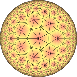
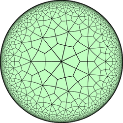
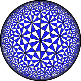
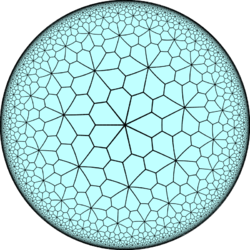
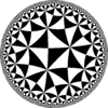
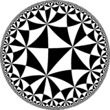
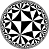
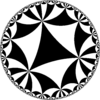
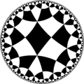
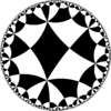
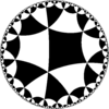
Hyperbolic groups in H2
| Example right triangles [p,q] | ||||
|---|---|---|---|---|
 [3,7] |
 [3,8] |
 [3,9] |
 [3,∞] | |
 [4,5] |
 [4,6] |
 [4,7] |
 [4,8] |
 [∞,4] |
 [5,5] |
 [5,6] |
 [5,7] |
 [6,6] |
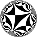 [∞,∞] |
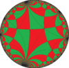
| Example general triangles [(p,q,r)] | ||||
 [(3,3,4)] |
 [(3,3,5)] |
 [(3,3,6)] |
 [(3,3,7)] |
 [(3,3,∞)] |
 [(3,4,4)] |
 [(3,6,6)] |
 [(3,∞,∞)] |
 [(6,6,6)] |
 [(∞,∞,∞)] |
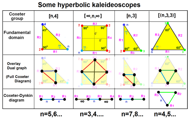
Two-dimensional hyperbolic triangle groups exist as rank 3 Coxeter diagrams, defined by triangle (p q r) for:

There are infinitely many compact triangular hyperbolic Coxeter groups, including linear and triangle graphs. The linear graphs exist for right triangles (with r=2).[5]
| Linear | Cyclic | ||||
|---|---|---|---|---|---|
| ∞ [p,q], 2(p+q)<pq
|
∞ [(p,q,r)],
|
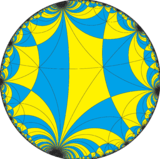
Paracompact Coxeter groups of rank 3 exist as limits to the compact ones.
| Linear graphs | Cyclic graphs |
|---|---|
|
|
Arithmetic triangle group
The hyperbolic triangle groups that are also arithmetic groups form a finite subset. By computer search the complete list was determined by Kisao Takeuchi in his 1977 paper Arithmetic triangle groups.[6] There are 85 total, 76 compact and 9 paracompact.
| Right triangles (p q 2) | General triangles (p q r) |
|---|---|
Compact groups: (76)
Paracompact right triangles: (4)
|
General triangles: (39)
Paracompact general triangles: (5)
|
|
|
Hyperbolic Coxeter polygons above triangles
 [∞,3,∞] [iπ/λ1,3,iπ/λ2] (*3222) |
 [((3,∞,3)),∞] [((3,iπ/λ1,3)),iπ/λ2] (*3322) |
 [(3,∞)[2]] [(3,iπ/λ1,3,iπ/λ2)] (*3232) |
 [(4,∞)[2]] [(4,iπ/λ1,4,iπ/λ2)] (*4242) |
 (*3333) |
| Domains with ideal vertices | ||||
|---|---|---|---|---|
 [iπ/λ1,∞,iπ/λ2] (*∞222) |
 (*∞∞22) |
 [(iπ/λ1,∞,iπ/λ2,∞)] (*2∞2∞) |
 (*∞∞∞∞) |
 (*4444) |
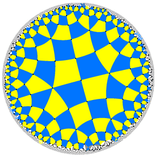
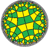
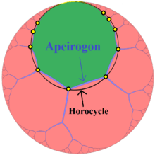
Other H2 hyperbolic kaleidoscopes can be constructed from higher order polygons. Like triangle groups these kaleidoscopes can be identified by a cyclic sequence of mirror intersection orders around the fundamental domain, as (a b c d ...), or equivalently in orbifold notation as *abcd.... Coxeter–Dynkin diagrams for these polygonal kaleidoscopes can be seen as a degenerate (n-1)-simplex fundamental domains, with a cyclic of branches order a,b,c... and the remaining n*(n-3)/2 branches are labeled as infinite (∞) representing the non-intersecting mirrors. The only nonhyperbolic example is Euclidean symmetry four mirrors in a square or rectangle as ![]()
![]()
![]()
![]()
![]()
![]()
![]() , [∞,2,∞] (orbifold *2222). Another branch representation for non-intersecting mirrors by Vinberg gives infinite branches as dotted or dashed lines, so this diagram can be shown as
, [∞,2,∞] (orbifold *2222). Another branch representation for non-intersecting mirrors by Vinberg gives infinite branches as dotted or dashed lines, so this diagram can be shown as ![]()
![]()
![]() , with the four order-2 branches suppressed around the perimeter.
, with the four order-2 branches suppressed around the perimeter.
For example, a quadrilateral domain (a b c d) will have two infinite order branches connecting ultraparallel mirrors. The smallest hyperbolic example is ![]()
![]()
![]()
![]()
![]()
![]()
![]() , [∞,3,∞] or [iπ/λ1,3,iπ/λ2] (orbifold *3222), where (λ1,λ2) are the distance between the ultraparallel mirrors. The alternate expression is
, [∞,3,∞] or [iπ/λ1,3,iπ/λ2] (orbifold *3222), where (λ1,λ2) are the distance between the ultraparallel mirrors. The alternate expression is ![]()
![]()
![]() , with three order-2 branches suppressed around the perimeter. Similarly (2 3 2 3) (orbifold *3232) can be represented as
, with three order-2 branches suppressed around the perimeter. Similarly (2 3 2 3) (orbifold *3232) can be represented as ![]()
![]()
![]() and (3 3 3 3), (orbifold *3333) can be represented as a complete graph
and (3 3 3 3), (orbifold *3333) can be represented as a complete graph ![]()
![]()
![]() .
.
The highest quadrilateral domain (∞ ∞ ∞ ∞) is an infinite square, represented by a complete tetrahedral graph with 4 perimeter branches as ideal vertices and two diagonal branches as infinity (shown as dotted lines) for ultraparallel mirrors: ![]()
![]()
![]()
![]()
![]() .
.
Compact (Lannér simplex groups)
Compact hyperbolic groups are called Lannér groups after Folke Lannér who first studied them in 1950.[7] They only exist as rank 4 and 5 graphs. Coxeter studied the linear hyperbolic coxeter groups in his 1954 paper Regular Honeycombs in hyperbolic space,[8] which included two rational solutions in hyperbolic 4-space: [5/2,5,3,3] = ![]()
![]()
![]()
![]()
![]()
![]()
![]()
![]()
![]()
![]()
![]() and [5,5/2,5,3] =
and [5,5/2,5,3] = ![]()
![]()
![]()
![]()
![]()
![]()
![]()
![]()
![]()
![]()
![]() .
.
Ranks 4–5
The fundamental domain of either of the two bifurcating groups, [5,31,1] and [5,3,31,1], is double that of a corresponding linear group, [5,3,4] and [5,3,3,4] respectively. Letter names are given by Johnson as extended Witt symbols.[9]
| Dimension Hd |
Rank | Total count | Linear | Bifurcating | Cyclic |
|---|---|---|---|---|---|
| H3 | 4 | 9 | = [4,3,5]: |
= [5,31,1]: |
= [(33,4)]: |
| H4 | 5 | 5 | = [33,5]: |
= [5,3,31,1]: |
= [(34,4)]: |


Paracompact (Koszul simplex groups)
Paracompact (also called noncompact) hyperbolic Coxeter groups contain affine subgroups and have asymptotic simplex fundamental domains. The highest paracompact hyperbolic Coxeter group is rank 10. These groups are named after French mathematician Jean-Louis Koszul.[10] They are also called quasi-Lannér groups extending the compact Lannér groups. The list was determined complete by computer search by M. Chein and published in 1969.[11]
By Vinberg, all but eight of these 72 compact and paracompact simplices are arithmetic. Two of the nonarithmetic groups are compact: ![]()
![]()
![]()
![]()
![]() and
and ![]()
![]()
![]()
![]()
![]()
![]() . The other six nonarithmetic groups are all paracompact, with five 3-dimensional groups
. The other six nonarithmetic groups are all paracompact, with five 3-dimensional groups ![]()
![]()
![]()
![]()
![]()
![]()
![]() ,
, ![]()
![]()
![]()
![]()
![]() ,
, ![]()
![]()
![]()
![]()
![]()
![]()
![]() ,
, ![]()
![]()
![]()
![]()
![]() , and
, and ![]()
![]()
![]()
![]()
![]() , and one 5-dimensional group
, and one 5-dimensional group ![]()
![]()
![]()
![]()
![]()
![]() .
.
Ideal simplices
There are 5 hyperbolic Coxeter groups expressing ideal simplices, graphs where removal of any one node results in an affine Coxeter group. Thus all vertices of this ideal simplex are at infinity.[12]
| Rank | Ideal group | Affine subgroups | ||
|---|---|---|---|---|
| 3 | [(∞,∞,∞)] | [∞] | ||
| 4 | [4[4]] | [4,4] | ||
| 4 | [3[3,3]] | [3[3]] | ||
| 4 | [(3,6)[2]] | [3,6] | ||
| 6 | [(3,3,4)[2]] | [4,3,3,4], [3,4,3,3] | ||
Ranks 4–10
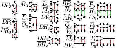
There are a total of 58 paracompact hyperbolic Coxeter groups from rank 4 through 10. All 58 are grouped below in five categories. Letter symbols are given by Johnson as Extended Witt symbols, using PQRSTWUV from the affine Witt symbols, and adding LMNOXYZ. These hyperbolic groups are given an overline, or a hat, for cycloschemes. The bracket notation from Coxeter is a linearized representation of the Coxeter group.
| Rank | Total count | Groups | |||
|---|---|---|---|---|---|
| 4 | 23 |
= [(3,3,4,4)]: |
= [3,3[3]]: |
= [3,4,4]: |
= [3[]x[]]: |
| 5 | 9 |
= [3,3[4]]: |
= [4,3,((4,2,3))]: |
= [(3,4)2]: |
= [4,31,1,1]: |
| 6 | 12 |
= [3,3[5]]: |
= [4,3,32,1]: |
= [33,4,3]: |
= [32,1,1,1]: = [4,3,31,1,1]: |
| 7 | 3 |
= [3,3[6]]: |
= [31,1,3,32,1]: |
= [4,32,32,1]: |
|
| 8 | 4 | = [3,3[7]]: |
= [31,1,32,32,1]: |
= [4,33,32,1]: |
= [33,2,2]: |
| 9 | 4 | = [3,3[8]]: |
= [31,1,33,32,1]: |
= [4,34,32,1]: |
= [34,3,1]: |
| 10 | 3 | = [ | = [31,1,34,32,1]: |
= [4,35,32,1]: |
= [36,2,1]: |


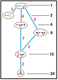
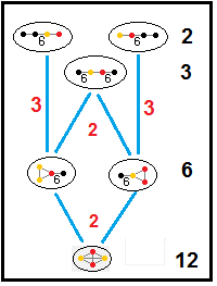
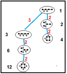
Subgroup relations of paracompact hyperbolic groups
These trees represents subgroup relations of paracompact hyperbolic groups. Subgroup indices on each connection are given in red.[13] Subgroups of index 2 represent a mirror removal, and fundamental domain doubling. Others can be inferred by commensurability (integer ratio of volumes) for the tetrahedral domains.
| H3 | 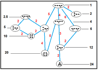 |
 |
 |
 |
|---|---|---|---|---|
| H4 | 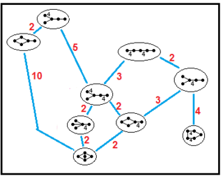 | |||
| H5 | 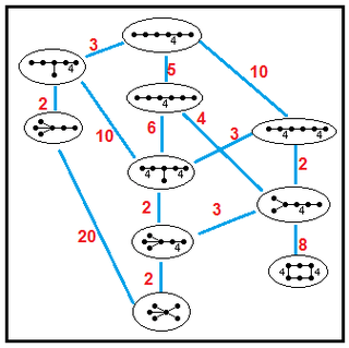 |
Hypercompact Coxeter groups (Vinberg polytopes)
Just like the hyperbolic plane H2 has nontriangular polygonal domains, higher-dimensional reflective hyperbolic domains also exists. These nonsimplex domains can be considered degenerate simplices with non-intersecting mirrors given infinite order, or in a Coxeter diagram, such branches are given dotted or dashed lines. These nonsimplex domains are called Vinberg polytopes, after Ernest Vinberg for his Vinberg's algorithm for finding nonsimplex fundamental domain of a hyperbolic reflection group. Geometrically these fundamental domains can be classified as quadrilateral pyramids, or prisms or other polytopes with edges as the intersection of two mirrors having dihedral angles as π/n for n=2,3,4...
In a simplex-based domain, there are n+1 mirrors for n-dimensional space. In non-simplex domains, there are more than n+1 mirrors. The list is finite, but not completely known. Instead partial lists have been enumerated as n+k mirrors for k as 2,3, and 4.
Hypercompact Coxeter groups in three dimensional space or higher differ from two dimensional groups in one essential respect. Two hyperbolic n-gons having the same angles in the same cyclic order may have different edge lengths and are not in general congruent. In contrast Vinberg polytopes in 3 dimensions or higher are completely determined by the dihedral angles. This fact is based on the Mostow rigidity theorem, that two isomorphic groups generated by reflections in Hn for n>=3, define congruent fundamental domains (Vinberg polytopes).
Vinberg polytopes with rank n+2 for n dimensional space
The complete list of compact hyperbolic Vinberg polytopes with rank n+2 mirrors for n-dimensions has been enumerated by F. Esselmann in 1996.[14] A partial list was published in 1974 by I. M. Kaplinskaya.[15]
The complete list of paracompact solutions was published by P. Tumarkin in 2003, with dimensions from 3 to 17.[16]
The smallest paracompact form in H3 can be represented by ![]()
![]()
![]()
![]()
![]()
![]()
![]()
![]()
![]() , or [∞,3,3,∞] which can be constructed by a mirror removal of paracompact hyperbolic group [3,4,4] as [3,4,1+,4]. The doubled fundamental domain changes from a tetrahedron into a quadrilateral pyramid. Another pyramids include [4,4,1+,4] = [∞,4,4,∞],
, or [∞,3,3,∞] which can be constructed by a mirror removal of paracompact hyperbolic group [3,4,4] as [3,4,1+,4]. The doubled fundamental domain changes from a tetrahedron into a quadrilateral pyramid. Another pyramids include [4,4,1+,4] = [∞,4,4,∞], ![]()
![]()
![]()
![]()
![]()
![]()
![]() =
= ![]()
![]()
![]()
![]()
![]()
![]()
![]()
![]()
![]() . Removing a mirror from some of the cyclic hyperbolic Coxeter graphs become bow-tie graphs: [(3,3,4,1+,4)] = [((3,∞,3)),((3,∞,3))] or
. Removing a mirror from some of the cyclic hyperbolic Coxeter graphs become bow-tie graphs: [(3,3,4,1+,4)] = [((3,∞,3)),((3,∞,3))] or ![]()
![]()
![]()
![]()
![]() , [(3,4,4,1+,4)] = [((4,∞,3)),((3,∞,4))] or
, [(3,4,4,1+,4)] = [((4,∞,3)),((3,∞,4))] or ![]()
![]()
![]()
![]()
![]() , [(4,4,4,1+,4)] = [((4,∞,4)),((4,∞,4))] or
, [(4,4,4,1+,4)] = [((4,∞,4)),((4,∞,4))] or ![]()
![]()
![]()
![]()
![]() .
.
Other valid paracompact graphs with quadrilateral pyramid fundamental domains include:
| Dimension | Rank | Graphs |
|---|---|---|
| H3 | 5 |
|
Another subgroup [1+,41,1,1] = [∞,4,1+,4,∞] = [∞[6]]. ![]()
![]()
![]()
![]()
![]() =
= ![]()
![]()
![]()
![]()
![]()
![]()
![]()
![]()
![]() =
= ![]()
![]()
![]()
![]()
![]()
![]()
![]() .
[17]
.
[17]
Vinberg polytopes with rank n+3 for n dimensional space
There are a finite number of degenerate fundamental simplices exist up to 8-dimensions. The complete list of Compact Vinberg polytopes with rank n+3 mirrors for n-dimensions has been enumerated by P. Tumarkin in 2004. These groups are labeled by dotted/broken lines for ultraparallel branches. The complete list of non-Compact Vinberg polytopes with rank n+3 mirrors and with one non-simple vertex for n-dimensions has been enumerated by Mike Roberts.[18]
For 4 to 8 dimensions, rank 7 to 11 Coxeter groups are counted as 44, 16, 3, 1, and 1 respectively.[19] The highest was discovered by Bugaenko in 1984 in dimension 8, rank 11:[20]
| Dimensions | Rank | Cases | Graphs | ||
|---|---|---|---|---|---|
| H4 | 7 | 44 | ... | ||
| H5 | 8 | 16 | .. | ||
| H6 | 9 | 3 | |||
| H7 | 10 | 1 | |||
| H8 | 11 | 1 | |||
Vinberg polytopes with rank n+4 for n dimensional space
There are a finite number of degenerate fundamental simplices exist up to 8-dimensions. Compact Vinberg polytopes with rank n+4 mirrors for n-dimensions has been explored by A. Felikson and P. Tumarkin in 2005.[21]
Lorentzian groups
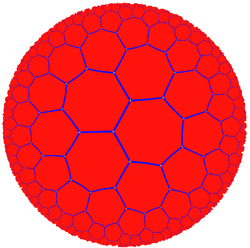
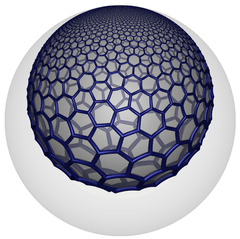
 {3,3,7} in hyperbolic 3-space, rendered the intersection of the honeycomb with the plane-at-infinity, in the Poincare half-space model. |
 {7,3,3} viewed outside of Poincare ball model. |

Lorentzian groups for simplex domains can be defined as graphs beyond the paracompact hyperbolic forms. These are sometimes called super-ideal simplices and are also related to a Lorentzian geometry, named after Hendrik Lorentz in the field of special and general relativity space-time, containing one (or more) time-like dimensional components whose self dot products are negative.[9] Danny Calegari calls these convex cocompact Coxeter groups in n-dimensional hyperbolic space.[22][23]
A 1982 paper by George Maxwell, Sphere Packings and Hyperbolic Reflection Groups, enumerates the finite list of Lorentzian of rank 5 to 11. He calls them level 2, meaning removal any permutation of 2 nodes leaves a finite or Euclidean graph. His enumeration is complete, but didn't list graphs that are a subgroup of another. All higher-order branch Coxeter groups of rank-4 are Lorentzian, ending in the limit as a complete graph 3-simplex Coxeter-Dynkin diagram with 6 infinite order branches, which can be expressed as [∞[3,3]]. Rank 5-11 have a finite number of groups 186, 66, 36, 13, 10, 8, and 4 Lorentzian groups respectively.[24] A 2013 paper by H. Chen and J.-P. Labbé, Lorentzian Coxeter groups and Boyd--Maxwell ball packings, recomputed and published the complete list.[25]
For the highest ranks 8-11, the complete lists are:
| Rank | Total count |
Groups | ||||
|---|---|---|---|---|---|---|
| 4 | ∞ | [3,3,7] ... [∞,∞,∞]: [4,3[3]] ... [∞,∞[3]]: | ||||
| 5 | 186 | ...[3[3,3,3]]: |
||||
| 6 | 66 | |||||
| 7 | 36 | [31,1,1,1,1,1]: | ||||
| 8 | 13 |
[3,3,3[6]]: |
[4,3,3,33,1]: |
[4,3,3,32,2]: | ||
| 9 | 10 |
[3,3[3+4],3]: |
[32,1,32,32,1]: |
[33,1,33,4]: [33,1,3,3,31,1]: |
[33,3,2]: [32,2,4]: | |
| 10 | 8 | [3,3[8],3]: [3,3[3+5],3]: |
[32,1,33,32,1]: |
[35,3,1]: [33,1,34,4]: |
[34,4,1]: | |
| 11 | 4 | [32,1,34,32,1]: |
[32,1,36,4]: [32,1,35,31,1]: |
[37,2,1]: | ||
Very-extended Coxeter Diagrams
One usage includes a very-extended definition from the direct Dynkin diagram usage which considers affine groups as extended, hyperbolic groups over-extended, and a third node as very-extended simple groups. These extensions are usually marked by an exponent of 1,2, or 3 + symbols for the number of extended nodes. This extending series can be extended backwards, by sequentially removing the nodes from the same position in the graph, although the process stops after removing branching node. The E8 extended family is the most commonly shown example extending backwards from E3 and forwards to E11.
The extending process can define a limited series of Coxeter graphs that progress from finite to affine to hyperbolic to Lorentzian. The determinant of the Cartan matrices determine where the series changes from finite (positive) to affine (zero) to hyperbolic (negative), and ending as a Lorentzian group, containing at least one hyperbolic subgroup.[26] The noncrystalographic Hn groups forms an extended series where H4 is extended as a compact hyperbolic and over-extended into a lorentzian group.
The determinant of the Schläfli matrix by rank are:[27]
- det(A1n=[2n-1]) = 2n (Finite for all n)
- det(An=[3n-1]) = n+1 (Finite for all n)
- det(Bn=[4,3n-2]) = 2 (Finite for all n)
- det(Dn=[3n-3,1,1]) = 4 (Finite for all n)
Determinants of the Schläfli matrix in exceptional series are:
- det(En=[3n-3,2,1]) = 9-n (Finite for E3(=A2A1), E4(=A4), E5(=D5), E6, E7 and E8, affine at E9 (), hyperbolic at E10)
- det([3n-4,3,1]) = 2(8-n) (Finite for n=4 to 7, affine (), and hyperbolic at n=8.)
- det([3n-4,2,2]) = 3(7-n) (Finite for n=4 to 6, affine (), and hyperbolic at n=7.)
- det(Fn=[3,4,3n-3]) = 5-n (Finite for F3(=B3) to F4, affine at F5 (), hyperbolic at F6)
- det(Gn=[6,3n-2]) = 3-n (Finite for G2, affine at G3 (), hyperbolic at G4)
| Finite | |||||||
|---|---|---|---|---|---|---|---|
| Rank n | [3[3],3n-3] | [4,4,3n-3] | Gn=[6,3n-2] | [3[4],3n-4] | [4,31,n-3] | [4,3,4,3n-4] | Hn=[5,3n-2] |
| 2 | [3] A2 |
[4] C2 |
[6] G2 |
[2] A12 |
[4] C2 |
[5] H2 | |
| 3 | [3[3]] A2+= |
[4,4] C2+= |
[6,3] G2+= |
[3,3]=A3 |
[4,3] B3 |
[4,3] C3 |
[5,3] H3 |
| 4 | [3[3],3] A2++= |
[4,4,3] C2++= |
[6,3,3] G2++= |
[3[4]] A3+= |
[4,31,1] B3+= |
[4,3,4] C3+= |
[5,3,3] H4 |
| 5 | [3[3],3,3] A2+++ |
[4,4,3,3] C2+++ |
[6,3,3,3] G2+++ |
[3[4],3] A3++= |
[4,32,1] B3++= |
[4,3,4,3] C3++= |
[5,33] H5= |
| 6 | [3[4],3,3] A3+++ |
[4,33,1] B3+++ |
[4,3,4,3,3] C3+++ |
[5,34] H6 | |||
| Det(Mn) | 3(3-n) | 2(3-n) | 3-n | 4(4-n) | 2(4-n) | ||


| Finite | ||||||||
|---|---|---|---|---|---|---|---|---|
| Rank n | [3[5],3n-5] | [4,3,3n-4,1] | [4,3,3,4,3n-5] | [3n-4,1,1,1] | [3,4,3n-3] | [3[6],3n-6] | [4,3,3,3n-5,1] | [31,1,3,3n-5,1] |
| 3 | [4,3−1,1] B2A1 |
[4,3] B3 |
[3−1,1,1,1] A13 |
[3,4] B3 |
[4,3,3] C3 | |||
| 4 | [33] A4 |
[4,3,3] B4 |
[4,3,3] C4 |
[30,1,1,1] D4 |
[3,4,3] F4 |
[4,3,3,3−1,1] B3A1 |
[31,1,3,3−1,1] A3A1 | |
| 5 | [3[5]] A4+= |
[4,3,31,1] B4+= |
[4,3,3,4] C4+= |
[31,1,1,1] D4+= |
[3,4,3,3] F4+= |
[34] A5 |
[4,3,3,3,3] B5 |
[31,1,3,3] D5 |
| 6 | [3[5],3] A4++= |
[4,3,32,1] B4++= |
[4,3,3,4,3] C4++= |
[32,1,1,1] D4++= |
[3,4,33] F4++= |
[3[6]] A5+= |
[4,3,3,31,1] B5+= |
[31,1,3,31,1] D5+= |
| 7 | [3[5],3,3] A4+++ |
[4,3,33,1] B4+++ |
[4,3,3,4,3,3] C4+++ |
[33,1,1,1] D4+++ |
[3,4,34] F4+++ |
[3[6],3] A5++= |
[4,3,3,32,1] B5++= |
[31,1,3,32,1] D5++= |
| 8 | [3[6],3,3] A5+++ |
[4,3,3,33,1] B5+++ |
[31,1,3,33,1] D5+++ | |||||
| Det(Mn) | 5(5-n) | 2(5-n) | 4(5-n) | 5-n | 6(6-n) | 4(6-n) | ||


| Finite | |||||||||
|---|---|---|---|---|---|---|---|---|---|
| Rank n | [3[7],3n-7] | [4,33,3n-6,1] | [31,1,3,3,3n-6,1] | [3n-5,2,2] | [3[8],3n-8] | [4,34,3n-7,1] | [31,1,3,3,3,3n-7,1] | [3n-5,3,1] | En=[3n-4,2,1] |
| 3 | [3−1,2,1] E3=A2A1 | ||||||||
| 4 | [3−1,2,2] A22 |
[3−1,3,1] A3A1 |
[30,2,1] E4=A4 | ||||||
| 5 | [4,3,3,3,3−1,1] B4A1 |
[31,1,3,3,3−1,1] D4A1 |
[30,2,2] A5 |
[30,3,1] A5 |
[31,2,1] E5=D5 | ||||
| 6 | [35] A6 |
[4,34] B6 |
[31,1,3,3,3] D6 |
[31,2,2] E6 |
[4,3,3,3,3,3−1,1] B5A1 |
[31,1,3,3,3,3−1,1] D5A1 |
[31,3,1] D6 |
[32,2,1] E6 * | |
| 7 | [3[7]] A6+= |
[4,33,31,1] B6+= |
[31,1,3,3,31,1] D6+= |
[32,2,2] E6+= |
[36] A7 |
[4,35] B7 |
[31,1,3,3,3,30,1] D7 |
[32,3,1] E7 * |
[33,2,1] E7 * |
| 8 | [3[7],3] A6++= |
[4,33,32,1] B6++= |
[31,1,3,3,32,1] D6++= |
[33,2,2] E6++= |
[3[8]] A7+= * |
[4,34,31,1] B7+= * |
[31,1,3,3,3,31,1] D7+= * |
[33,3,1] E7+= * |
[34,2,1] E8 * |
| 9 | [3[7],3,3] A6+++ |
[4,33,33,1] B6+++ |
[31,1,3,3,33,1] D6+++ |
[34,2,2] E6+++ |
[3[8],3] A7++= * |
[4,34,32,1] B7++= * |
[31,1,3,3,3,32,1] D7++= * |
[34,3,1] E7++= * |
[35,2,1] E9=E8+= * |
| 10 | [3[8],3,3] A7+++ * |
[4,34,33,1] B7+++ * |
[31,1,3,3,3,33,1] D7+++ * |
[35,3,1] E7+++ * |
[36,2,1] E10=E8++= * | ||||
| 11 | [37,2,1] E11=E8+++ * | ||||||||
| Det(Mn) | 7(7-n) | 2(7-n) | 4(7-n) | 3(7-n) | 8(8-n) | 2(8-n) | 4(8-n) | 2(8-n) | 9-n |


Geometric folding
| φA : AΓ --> AΓ' for finite types | |||
|---|---|---|---|
| Γ | Γ' | Folding description | Coxeter–Dynkin diagrams |
| I2(h) | Γ(h) | Dihedral folding |  |
| Bn | A2n | (I,sn) | |
| Dn+1, A2n-1 | (A3,+/-ε) | ||
| F4 | E6 | (A3,±ε) | |
| H4 | E8 | (A4,±ε) | |
| H3 | D6 | ||
| H2 | A4 | ||
| G2 | A5 | (A5,±ε) | |
| D4 | (D4,±ε) | ||
| φ: AΓ+ --> AΓ'+ for affine types | |||
| Locally trivial |  | ||
| (I,sn) | |||
| , | (A3,±ε) | ||
| , | (A3,±ε) | ||
| (I,sn) | |||
| (I,sn) & (I,s0) | |||
| (A3,ε) & (I,s0) | |||
| (A3,ε) & (A3,ε') | |||
| (A3,-ε) & (A3,-ε') | |||
| (I,s1) | |||
| , | (A3,±ε) | ||
| , | (A5,±ε) | ||
| , | (B3,±ε) | ||
| , | (D4,±ε) | ||


A (simply-laced) Coxeter–Dynkin diagram (finite, affine, or hyperbolic) that has a symmetry (satisfying one condition, below) can be quotiented by the symmetry, yielding a new, generally multiply laced diagram, with the process called "folding".[29][30]
For example, in D4 folding to G2, the edge in G2 points from the class of the 3 outer nodes (valence 1), to the class of the central node (valence 3).
Geometrically this corresponds to orthogonal projections of uniform polytopes and tessellations. Notably, any finite simply-laced Coxeter–Dynkin diagram can be folded to I2(h), where h is the Coxeter number, which corresponds geometrically to a projection to the Coxeter plane.
 A few hyperbolic foldings |
Complex reflections
Coxeter-Dynkin diagram has been extended to Complex space, Cn where nodes are unitary reflections of period greater than 2. Nodes are labeled by an index, assumed to be 2 for ordinary real reflection if suppressed. Coxeter writes the complex group, p[q]r, as diagram ![]()
![]()
![]()
![]()
![]() . [31]
. [31]
A 1-dimensional regular complex polytope in is represented as ![]() , having p vertices. Its real representation is a regular polygon, {p}. Its symmetry is p[] or
, having p vertices. Its real representation is a regular polygon, {p}. Its symmetry is p[] or ![]() , order p. A unitary operator generator for
, order p. A unitary operator generator for ![]() is seen as a rotation in by 2π/p radians counter clockwise, and a
is seen as a rotation in by 2π/p radians counter clockwise, and a ![]() edge is created by sequential applications of a single unitary reflection. A unitary reflection generator for a 1-polytope with p vertices is e2πi/p = cos(2π/p) + i sin(2π/p). When p = 2, the generator is eπi = –1, the same as a point reflection in the real plane.
edge is created by sequential applications of a single unitary reflection. A unitary reflection generator for a 1-polytope with p vertices is e2πi/p = cos(2π/p) + i sin(2π/p). When p = 2, the generator is eπi = –1, the same as a point reflection in the real plane.


In a higher polytope, p{} or ![]() represents a p-edge element, with a 2-edge, {} or
represents a p-edge element, with a 2-edge, {} or ![]() , representing an ordinary real edge between two vertices.
, representing an ordinary real edge between two vertices.
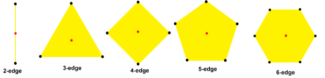 Complex 1-polytopes represented in the Argand plane as regular polygons for p = 2, 3, 4, 5, and 6, with black vertices. The centroid of the p vertices is shown seen in red. The sides of the polygons represent one application of the symmetry generator, mapping each vertex to the next counterclockwise copy. These polygonal sides are not edge elements of the polytope, as a complex 1-polytope can have no edges (it often is a complex edge) and only contains vertex elements. |
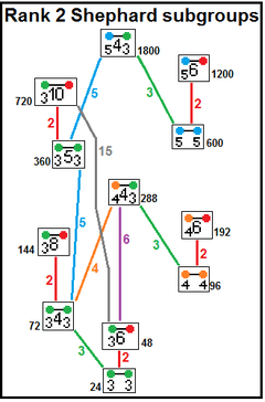 12 irreducible Shephard groups with their subgroup index relations.[32] Subgroups index 2 relate by removing a real reflection: p[2q]2 --> p[q]p, index 2. p[4]q --> p[q]p, index q. |
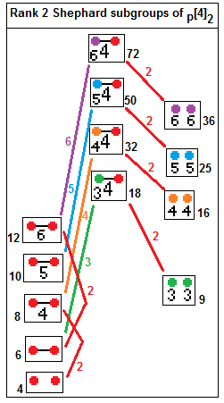 p[4]2 subgroups: p=2,3,4... p[4]2 --> [p], index p p[4]2 --> p[]×p[], index 2 |
Aa regular complex polygons in , has the form p{q}r or Coxeter diagram ![]()
![]()
![]()
![]()
![]() . The symmetry group of a regular complex polygon
. The symmetry group of a regular complex polygon ![]()
![]()
![]()
![]()
![]() is not called a Coxeter group, but instead a Shephard group, a type of Complex reflection group. The order of p[q]r is .[33]
is not called a Coxeter group, but instead a Shephard group, a type of Complex reflection group. The order of p[q]r is .[33]


The rank 2 Shephard groups are: 2[q]2, p[4]2, 3[3]3, 3[6]2, 3[4]3, 4[3]4, 3[8]2, 4[6]2, 4[4]3, 3[5]3, 5[3]5, 3[10]2, 5[6]2, and 5[4]3 or ![]()
![]()
![]() ,
, ![]()
![]()
![]() ,
, ![]()
![]()
![]() ,
, ![]()
![]()
![]() ,
, ![]()
![]()
![]() ,
, ![]()
![]()
![]() ,
, ![]()
![]()
![]() ,
, ![]()
![]()
![]() ,
, ![]()
![]()
![]() ,
, ![]()
![]()
![]() ,
, ![]()
![]()
![]() ,
, ![]()
![]()
![]() ,
, ![]()
![]()
![]() ,
, ![]()
![]()
![]() of order 2q, 2p2, 24, 48, 72, 96, 144, 192, 288, 360, 600, 1200, and 1800 respectively.
of order 2q, 2p2, 24, 48, 72, 96, 144, 192, 288, 360, 600, 1200, and 1800 respectively.
The symmetry group p1[q]p2 is represented by 2 generators R1, R2, where: R1p1 = R2p2 = I. If q is even, (R2R1)q/2 = (R1R2)q/2. If q is odd, (R2R1)(q-1)/2R2 = (R1R2)(q-1)/2R1. When q is odd, p1=p2.
The group ![]()
![]()
![]() or [1 1 1]p is defined by 3 period 2 unitary reflections {R1, R2, R3}: R12 = R12 = R32 = (R1R2)3 = (R2R3)3 = (R3R1)3 = (R1R2R3R1)p = 1. The period p can be seen as a double rotation in real .
or [1 1 1]p is defined by 3 period 2 unitary reflections {R1, R2, R3}: R12 = R12 = R32 = (R1R2)3 = (R2R3)3 = (R3R1)3 = (R1R2R3R1)p = 1. The period p can be seen as a double rotation in real .


A similar group ![]()
![]()
![]() or [1 1 1](p) is defined by 3 period 2 unitary reflections {R1, R2, R3}: R12 = R12 = R32 = (R1R2)3 = (R2R3)3 = (R3R1)3 = (R1R2R3R2)p = 1.
or [1 1 1](p) is defined by 3 period 2 unitary reflections {R1, R2, R3}: R12 = R12 = R32 = (R1R2)3 = (R2R3)3 = (R3R1)3 = (R1R2R3R2)p = 1.
See also
- Coxeter group
- Schwarz triangle
- Goursat tetrahedron
- Dynkin diagram
- Uniform polytope
- Wythoff construction and Wythoff symbol
References
- ↑ Hall, Brian C. (2003), Lie Groups, Lie Algebras, and Representations: An Elementary Introduction, Springer, ISBN 0-387-40122-9
- ↑ Coxeter, Regular Polytopes, (3rd edition, 1973), Dover edition, ISBN 0-486-61480-8, Sec 7.7. page 133, Schläfli's Criterion
- ↑ Lannér F., On complexes with transitive groups of automorphisms, Medd. Lunds Univ. Mat. Sem. [Comm. Sem. Math. Univ. Lund], 11 (1950), 1–71
- ↑ Allcock, Daniel (11 July 2006). "Infinitely many hyperbolic Coxeter groups through dimension 19". Geometry & Topology. 10: 737–758. doi:10.2140/gt.2006.10.737.
- ↑ The Geometry and Topology of Coxeter Groups, Michael W. Davis, 2008 p. 105 Table 6.2. Hyperbolic diagrams
- ↑ "TAKEUCHI : Arithmetic triangle groups". Projecteuclid.org. Retrieved 2013-07-05.
- ↑ Folke Lannér, On complexes with transitive groups of automorphisms, Comm. Sém., Math. Univ. Lund [Medd. Lunds Univ. Mat. Sem.] 11 (1950)
- ↑ Regular Honeycombs in hyperbolic space, Coxeter, 1954
- 1 2 Norman Johnson, Geometries and Transformations, Chapter 13: Hyperbolic Coxeter groups, 13.6 Lorentzian lattices
- ↑ J. L. Koszul, Lectures on hyperbolic Coxeter groups, University of Notre Dame (1967)
- ↑ M. Chein, Recherche des graphes des matrices de Coxeter hyperboliques d’ordre ≤10, Rev. Française Informat. Recherche Opérationnelle 3 (1969), no. Ser. R-3, 3–16 (French).
- ↑ Subalgebras of hyperbolic Kay-Moody algebras, Figure 5.1, p.13
- ↑ N.W. Johnson, R. Kellerhals, J.G. Ratcliffe,S.T. Tschantz, Commensurability classes of hyperbolic Coxeter groups H3: p130, H4: p137, H5: p 138.
- ↑ F. Esselmann, The classification of compact hyperbolic Coxeter d-polytopes with d+2 facets. Comment. Math. Helvetici 71 (1996), 229–242.
- ↑ I. M. Kaplinskaya, Discrete groups generated by reflections in the faces of simplicial prisms in Lobachevskian spaces. Math. Notes,15 (1974), 88–91.
- ↑ P. Tumarkin, Hyperbolic Coxeter n-polytopes with n+2 facets (2003)
- ↑ Norman W. Johnson and Asia Ivic Weiss, Quadratic Integers and Coxeter Groups, Canad. J. Math. Vol. 51 (6), 1999 pp. 1307–1336
- ↑ A Classification of Non-Compact Coxeter Polytopes with n+3 Facets and One Non-Simple Vertex
- ↑ P. Tumarkin, Compact hyperbolic Coxeter (2004)
- ↑ V. O. Bugaenko, Groups of automorphisms of unimodular hyperbolic quadratic forms over the ring Zh√5+12 i. Moscow Univ. Math. Bull. 39 (1984), 6-14.
- ↑ Anna Felikson, Pavel Tumarkin, On compact hyperbolic Coxeter d-polytopes with d+4 facets, 2005
- ↑ Random groups, diamonds and glass, Danny Calegari of the University of Chicago, June 25, 2014 at the Bill Thurston Legacy Conference
- ↑ Coxeter groups and random groups, Danny Calegari, last revised 4 Apr 2015
- ↑ George Maxwell, Sphere Packings and Hyperbolic Reflection Groups, JOURNAL OF ALGEBRA 79,78-97 (1982)
- ↑ Hao Chen, Jean-Philippe Labbé, Lorentzian Coxeter groups and Boyd-Maxwell ball packings, http://arxiv.org/abs/1310.8608
- ↑ Kac-Moody Algebras in M-theory
- ↑ Cartan–Gram determinants for the simple Lie groups, Wu, Alfred C. T, The American Institute of Physics, Nov 1982
- ↑ John Crisp, 'Injective maps between Artin groups', in Down under group theory, Proceedings of the Special Year on Geometric Group Theory, (Australian National University, Canberra, Australia, 1996), Postscript, pp 13-14, and googlebook, Geometric group theory down under, p 131
- ↑ Zuber, Jean-Bernard. "Generalized Dynkin diagrams and root systems and their folding": 28–30. CiteSeerX 10.1.1.54.3122
 .
. - ↑ Dechant, Pierre-Philippe; Boehm, Celine; Twarock, Reidun (October 25, 2011). "Affine extensions of non-crystallographic Coxeter groups induced by projection". arXiv:1110.5228.
- ↑ Coxeter, Complex Regular Polytopes, second edition, (1991)
- ↑ Coxeter, Complex Regular Polytopes, p. 177, Table III
- ↑ Unitary Reflection Groups, p.87
Further reading
- James E. Humphreys, Reflection Groups and Coxeter Groups, Cambridge studies in advanced mathematics, 29 (1990)
- Kaleidoscopes: Selected Writings of H.S.M. Coxeter, edited by F. Arthur Sherk, Peter McMullen, Anthony C. Thompson, Asia Ivic Weiss, Wiley-Interscience Publication, 1995, ISBN 978-0-471-01003-6 , Googlebooks
- (Paper 17) Coxeter, The Evolution of Coxeter-Dynkin diagrams, [Nieuw Archief voor Wiskunde 9 (1991) 233-248]
- Coxeter, The Beauty of Geometry: Twelve Essays, Dover Publications, 1999, ISBN 978-0-486-40919-1 (Chapter 3: Wythoff's Construction for Uniform Polytopes)
- Coxeter, Regular Polytopes (1963), Macmillian Company
- Regular Polytopes, Third edition, (1973), Dover edition, ISBN 0-486-61480-8 (Chapter 5: The Kaleidoscope, and Section 11.3 Representation by graphs)
- H.S.M. Coxeter and W. O. J. Moser. Generators and Relations for Discrete Groups 4th ed, Springer-Verlag. New York. 1980
- Norman Johnson, Geometries and Transformations, Chapters 11,12,13, preprint 2011
- N. W. Johnson, R. Kellerhals, J. G. Ratcliffe, S. T. Tschantz, The size of a hyperbolic Coxeter simplex, Transformation Groups 1999, Volume 4, Issue 4, pp 329–353
- Norman W. Johnson and Asia Ivic Weiss Quadratic Integers and Coxeter Groups PDF Canad. J. Math. Vol. 51 (6), 1999 pp. 1307–1336
External links
- October 1978 discussion on the history of the Coxeter diagrams by Coxeter and Dynkin in Toronto, Canada; Eugene Dynkin Collection of Mathematics Interviews, Cornell University Library.