Standard deviation
In statistics, the standard deviation (SD, also represented by the Greek letter sigma σ or the Latin letter s) is a measure that is used to quantify the amount of variation or dispersion of a set of data values.[1] A low standard deviation indicates that the data points tend to be close to the mean (also called the expected value) of the set, while a high standard deviation indicates that the data points are spread out over a wider range of values.
The standard deviation of a random variable, statistical population, data set, or probability distribution is the square root of its variance. It is algebraically simpler, though in practice less robust, than the average absolute deviation.[2][3] A useful property of the standard deviation is that, unlike the variance, it is expressed in the same units as the data. There are also other measures of deviation from the norm, including mean absolute deviation, which provide different mathematical properties from standard deviation.[4]
In addition to expressing the variability of a population, the standard deviation is commonly used to measure confidence in statistical conclusions. For example, the margin of error in polling data is determined by calculating the expected standard deviation in the results if the same poll were to be conducted multiple times. This derivation of a standard deviation is often called the "standard error" of the estimate or "standard error of the mean" when referring to a mean. It is computed as the standard deviation of all the means that would be computed from that population if an infinite number of samples were drawn and a mean for each sample were computed. It is very important to note that the standard deviation of a population and the standard error of a statistic derived from that population (such as the mean) are quite different but related (related by the inverse of the square root of the number of observations). The reported margin of error of a poll is computed from the standard error of the mean (or alternatively from the product of the standard deviation of the population and the inverse of the square root of the sample size, which is the same thing) and is typically about twice the standard deviation—the half-width of a 95 percent confidence interval. In science, researchers commonly report the standard deviation of experimental data, and only effects that fall much farther than two standard deviations away from what would have been expected are considered statistically significant—normal random error or variation in the measurements is in this way distinguished from likely genuine effects or associations. The standard deviation is also important in finance, where the standard deviation on the rate of return on an investment is a measure of the volatility of the investment.
When only a sample of data from a population is available, the term standard deviation of the sample or sample standard deviation can refer to either the above-mentioned quantity as applied to those data or to a modified quantity that is an unbiased estimate of the population standard deviation (the standard deviation of the entire population).
Basic examples
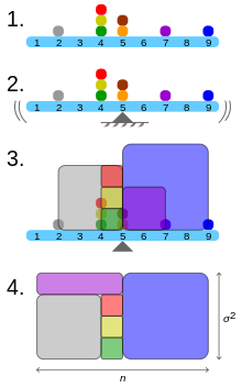
- A frequency distribution is constructed.
- The centroid of the distribution gives its mean.
- A square with sides equal to the difference of each value from the mean is formed for each value.
- Arranging the squares into a rectangle with one side equal to the number of values, n, results in the other side being the distribution's variance, σ².
For a finite set of numbers, the standard deviation is found by taking the square root of the average of the squared deviations of the values from their average value. For example, the marks of a class of eight students (that is, a population) are the following eight values:

These eight data points have the mean (average) of 5:

First, calculate the deviations of each data point from the mean, and square the result of each:

The variance is the mean of these values:

and the population standard deviation is equal to the square root of the variance:

This formula is valid only if the eight values with which we began form the complete population. If the values instead were a random sample drawn from some large parent population (for example, they were 8 marks randomly and independently chosen from a class of 2 million), then one often divides by 7 (which is n − 1) instead of 8 (which is n) in the denominator of the last formula. In that case the result would be called the sample standard deviation. Dividing by n − 1 rather than by n gives an unbiased estimate of the standard deviation of the larger parent population. This is known as Bessel's correction.[5]
As a slightly more complicated real-life example, the average height for adult men in the United States is about 70 inches, with a standard deviation of around 3 inches. This means that most men (about 68%, assuming a normal distribution) have a height within 3 inches of the mean (67–73 inches) – one standard deviation – and almost all men (about 95%) have a height within 6 inches of the mean (64–76 inches) – two standard deviations. If the standard deviation were zero, then all men would be exactly 70 inches tall. If the standard deviation were 20 inches, then men would have much more variable heights, with a typical range of about 50–90 inches. Three standard deviations account for 99.7% of the sample population being studied, assuming the distribution is normal (bell-shaped). (See the 68-95-99.7 rule, or the empirical rule, for more information.)
Definition of population values
Let X be a random variable with mean value μ:
![\operatorname {E} [X]=\mu .\,\!](../I/m/a850f6d56e315eaef8b630976d5164b368ecb072.svg)
Here the operator E denotes the average or expected value of X. Then the standard deviation of X is the quantity
![{\displaystyle {\begin{aligned}\sigma &={\sqrt {\operatorname {E} [(X-\mu )^{2}]}}\\&={\sqrt {\operatorname {E} [X^{2}]+\operatorname {E} [-2\mu X]+\operatorname {E} [\mu ^{2}]}}={\sqrt {\operatorname {E} [X^{2}]-2\mu \operatorname {E} [X]+\mu ^{2}}}\\&={\sqrt {\operatorname {E} [X^{2}]-2\mu ^{2}+\mu ^{2}}}={\sqrt {\operatorname {E} [X^{2}]-\mu ^{2}}}\\&={\sqrt {\operatorname {E} [X^{2}]-(\operatorname {E} [X])^{2}}}\end{aligned}}}](../I/m/6d5e98f44504dd173af145ff80cda7cfd80d3050.svg)
(derived using the properties of expected value).
In other words, the standard deviation σ (sigma) is the square root of the variance of X; i.e., it is the square root of the average value of (X − μ)2.
The standard deviation of a (univariate) probability distribution is the same as that of a random variable having that distribution. Not all random variables have a standard deviation, since these expected values need not exist. For example, the standard deviation of a random variable that follows a Cauchy distribution is undefined because its expected value μ is undefined.
Discrete random variable
In the case where X takes random values from a finite data set x1, x2, ..., xN, with each value having the same probability, the standard deviation is
![\sigma ={\sqrt {{\frac {1}{N}}\left[(x_{1}-\mu )^{2}+(x_{2}-\mu )^{2}+\cdots +(x_{N}-\mu )^{2}\right]}},{\rm {\ \ where\ \ }}\mu ={\frac {1}{N}}(x_{1}+\cdots +x_{N}),](../I/m/2845de27edc898d2a2a4320eda5f57e0dac6f650.svg)
or, using summation notation,

If, instead of having equal probabilities, the values have different probabilities, let x1 have probability p1, x2 have probability p2, ..., xN have probability pN. In this case, the standard deviation will be

Continuous random variable
The standard deviation of a continuous real-valued random variable X with probability density function p(x) is

and where the integrals are definite integrals taken for x ranging over the set of possible values of the random variable X.
In the case of a parametric family of distributions, the standard deviation can be expressed in terms of the parameters. For example, in the case of the log-normal distribution with parameters μ and σ2, the standard deviation is [(exp(σ2) − 1)exp(2μ + σ2)]1/2.
Estimation
One can find the standard deviation of an entire population in cases (such as standardized testing) where every member of a population is sampled. In cases where that cannot be done, the standard deviation σ is estimated by examining a random sample taken from the population and computing a statistic of the sample, which is used as an estimate of the population standard deviation. Such a statistic is called an estimator, and the estimator (or the value of the estimator, namely the estimate) is called a sample standard deviation, and is denoted by s (possibly with modifiers). However, unlike in the case of estimating the population mean, for which the sample mean is a simple estimator with many desirable properties (unbiased, efficient, maximum likelihood), there is no single estimator for the standard deviation with all these properties, and unbiased estimation of standard deviation is a very technically involved problem. Most often, the standard deviation is estimated using the corrected sample standard deviation (using N − 1), defined below, and this is often referred to as the "sample standard deviation", without qualifiers. However, other estimators are better in other respects: the uncorrected estimator (using N) yields lower mean squared error, while using N − 1.5 (for the normal distribution) almost completely eliminates bias.
Uncorrected sample standard deviation
Firstly, the formula for the population standard deviation (of a finite population) can be applied to the sample, using the size of the sample as the size of the population (though the actual population size from which the sample is drawn may be much larger). This estimator, denoted by sN, is known as the uncorrected sample standard deviation, or sometimes the standard deviation of the sample (considered as the entire population), and is defined as follows:

where are the observed values of the sample items and is the mean value of these observations, while the denominator N stands for the size of the sample: this is the square root of the sample variance, which is the average of the squared deviations about the sample mean.


This is a consistent estimator (it converges in probability to the population value as the number of samples goes to infinity), and is the maximum-likelihood estimate when the population is normally distributed. However, this is a biased estimator, as the estimates are generally too low. The bias decreases as sample size grows, dropping off as 1/n, and thus is most significant for small or moderate sample sizes; for the bias is below 1%. Thus for very large sample sizes, the uncorrected sample standard deviation is generally acceptable. This estimator also has a uniformly smaller mean squared error than the corrected sample standard deviation.

Corrected sample standard deviation
If the biased sample variance (the second central moment of the sample, which is a downward-biased estimate of the population variance) is used to compute an estimate of the population's standard deviation, the result is

Here taking the square root introduces further downward bias, by Jensen's inequality, due to the square root being a concave function. The bias in the variance is easily corrected, but the bias from the square root is more difficult to correct, and depends on the distribution in question.
An unbiased estimator for the variance is given by applying Bessel's correction, using N − 1 instead of N to yield the unbiased sample variance, denoted s2:

This estimator is unbiased if the variance exists and the sample values are drawn independently with replacement. N − 1 corresponds to the number of degrees of freedom in the vector of deviations from the mean,

Taking square roots reintroduces bias (because the square root is a nonlinear function, which does not commute with the expectation), yielding the corrected sample standard deviation, denoted by s:

As explained above, while s2 is an unbiased estimator for the population variance, s is still a biased estimator for the population standard deviation, though markedly less biased than the uncorrected sample standard deviation. The bias is still significant for small samples (N less than 10), and also drops off as 1/N as sample size increases. This estimator is commonly used and generally known simply as the "sample standard deviation".
Unbiased sample standard deviation
For unbiased estimation of standard deviation, there is no formula that works across all distributions, unlike for mean and variance. Instead, s is used as a basis, and is scaled by a correction factor to produce an unbiased estimate. For the normal distribution, an unbiased estimator is given by s/c4, where the correction factor (which depends on N) is given in terms of the Gamma function, and equals:

This arises because the sampling distribution of the sample standard deviation follows a (scaled) chi distribution, and the correction factor is the mean of the chi distribution.
An approximation can be given by replacing N − 1 with N − 1.5, yielding:

The error in this approximation decays quadratically (as 1/N2), and it is suited for all but the smallest samples or highest precision: for n = 3 the bias is equal to 1.3%, and for n = 9 the bias is already less than 0.1%.
For other distributions, the correct formula depends on the distribution, but a rule of thumb is to use the further refinement of the approximation:

where γ2 denotes the population excess kurtosis. The excess kurtosis may be either known beforehand for certain distributions, or estimated from the data.
Confidence interval of a sampled standard deviation
The standard deviation we obtain by sampling a distribution is itself not absolutely accurate, both for mathematical reasons (explained here by the confidence interval) and for practical reasons of measurement (measurement error). The mathematical effect can be described by the confidence interval or CI. To show how a larger sample will make the confidence interval narrower, consider the following examples: A small population of N = 2 has only 1 degree of freedom for estimating the standard deviation. The result is that a 95% CI of the SD runs from 0.45*SD to 31.9*SD; the factors here are as follows:

where is the p-th quantile of the chi-square distribution with k degrees of freedom, and is the confidence level. This is equivalent to the following:


With k = 1, = 0.000982 and = 5.024. The reciprocals of the square roots of these two numbers give us the factors 0.45 and 31.9 given above.


A larger population of N = 10 has 9 degrees of freedom for estimating the standard deviation. The same computations as above give us in this case a 95% CI running from 0.69*SD to 1.83*SD. So even with a sample population of 10, the actual SD can still be almost a factor 2 higher than the sampled SD. For a sample population N=100, this is down to 0.88*SD to 1.16*SD. To be more certain that the sampled SD is close to the actual SD we need to sample a large number of points.
These same formulae can be used to obtain confidence intervals on the variance of residuals from a least squares fit under standard normal theory, where k is now the number of degrees of freedom for error.
Identities and mathematical properties
The standard deviation is invariant under changes in location, and scales directly with the scale of the random variable. Thus, for a constant c and random variables X and Y:


The standard deviation of the sum of two random variables can be related to their individual standard deviations and the covariance between them:

where and stand for variance and covariance, respectively.


The calculation of the sum of squared deviations can be related to moments calculated directly from the data. In the following formula, the letter E is interpreted to mean expected value, i.e., mean.
![\sigma (X)={\sqrt {E[(X-E(X))^{2}]}}={\sqrt {E[X^{2}]-(E[X])^{2}}}.](../I/m/c5ac32b768e8f2755b5fd8cfc2981a54df4936d9.svg)
The sample standard deviation can be computed as:
![\sigma (X)={\sqrt {\frac {N}{N-1}}}{\sqrt {E[(X-E(X))^{2}]}}.](../I/m/ab28a10b21bddd32e57d4c82dc2dcf6d08ab4d52.svg)
For a finite population with equal probabilities at all points, we have

This means that the standard deviation is equal to the square root of the difference between the average of the squares of the values and the square of the average value. See computational formula for the variance for proof, and for an analogous result for the sample standard deviation.
Interpretation and application
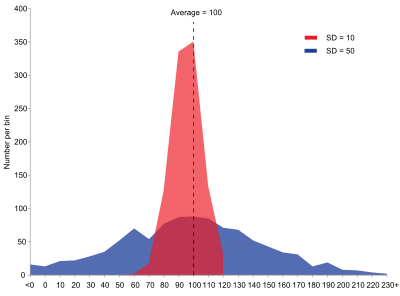
A large standard deviation indicates that the data points can spread far from the mean and a small standard deviation indicates that they are clustered closely around the mean.
For example, each of the three populations {0, 0, 14, 14}, {0, 6, 8, 14} and {6, 6, 8, 8} has a mean of 7. Their standard deviations are 7, 5, and 1, respectively. The third population has a much smaller standard deviation than the other two because its values are all close to 7. It will have the same units as the data points themselves. If, for instance, the data set {0, 6, 8, 14} represents the ages of a population of four siblings in years, the standard deviation is 5 years. As another example, the population {1000, 1006, 1008, 1014} may represent the distances traveled by four athletes, measured in meters. It has a mean of 1007 meters, and a standard deviation of 5 meters.
Standard deviation may serve as a measure of uncertainty. In physical science, for example, the reported standard deviation of a group of repeated measurements gives the precision of those measurements. When deciding whether measurements agree with a theoretical prediction, the standard deviation of those measurements is of crucial importance: if the mean of the measurements is too far away from the prediction (with the distance measured in standard deviations), then the theory being tested probably needs to be revised. This makes sense since they fall outside the range of values that could reasonably be expected to occur, if the prediction were correct and the standard deviation appropriately quantified. See prediction interval.
While the standard deviation does measure how far typical values tend to be from the mean, other measures are available. An example is the mean absolute deviation, which might be considered a more direct measure of average distance, compared to the root mean square distance inherent in the standard deviation.
Application examples
The practical value of understanding the standard deviation of a set of values is in appreciating how much variation there is from the average (mean).
Experiment, industrial and hypothesis testing
Standard deviation is often used to compare real-world data against a model to test the model. For example, in industrial applications the weight of products coming off a production line may need to comply with a legally required value. By weighing some fraction of the products an average weight can be found, which will always be slightly different to the long-term average. By using standard deviations, a minimum and maximum value can be calculated that the averaged weight will be within some very high percentage of the time (99.9% or more). If it falls outside the range then the production process may need to be corrected. Statistical tests such as these are particularly important when the testing is relatively expensive. For example, if the product needs to be opened and drained and weighed, or if the product was otherwise used up by the test.
In experimental science, a theoretical model of reality is used. Particle physics conventionally uses a standard of "5 sigma" for the declaration of a discovery.[6] A five-sigma level translates to one chance in 3.5 million that a random fluctuation would yield the result. This level of certainty was required in order to assert that a particle consistent with the Higgs boson had been discovered in two independent experiments at CERN,[7] and this was also the significance level leading to the declaration of the first detection of gravitational waves.[8]
Weather
As a simple example, consider the average daily maximum temperatures for two cities, one inland and one on the coast. It is helpful to understand that the range of daily maximum temperatures for cities near the coast is smaller than for cities inland. Thus, while these two cities may each have the same average maximum temperature, the standard deviation of the daily maximum temperature for the coastal city will be less than that of the inland city as, on any particular day, the actual maximum temperature is more likely to be farther from the average maximum temperature for the inland city than for the coastal one.
Finance
In finance, standard deviation is often used as a measure of the risk associated with price-fluctuations of a given asset (stocks, bonds, property, etc.), or the risk of a portfolio of assets[9] (actively managed mutual funds, index mutual funds, or ETFs). Risk is an important factor in determining how to efficiently manage a portfolio of investments because it determines the variation in returns on the asset and/or portfolio and gives investors a mathematical basis for investment decisions (known as mean-variance optimization). The fundamental concept of risk is that as it increases, the expected return on an investment should increase as well, an increase known as the risk premium. In other words, investors should expect a higher return on an investment when that investment carries a higher level of risk or uncertainty. When evaluating investments, investors should estimate both the expected return and the uncertainty of future returns. Standard deviation provides a quantified estimate of the uncertainty of future returns.
For example, assume an investor had to choose between two stocks. Stock A over the past 20 years had an average return of 10 percent, with a standard deviation of 20 percentage points (pp) and Stock B, over the same period, had average returns of 12 percent but a higher standard deviation of 30 pp. On the basis of risk and return, an investor may decide that Stock A is the safer choice, because Stock B's additional two percentage points of return is not worth the additional 10 pp standard deviation (greater risk or uncertainty of the expected return). Stock B is likely to fall short of the initial investment (but also to exceed the initial investment) more often than Stock A under the same circumstances, and is estimated to return only two percent more on average. In this example, Stock A is expected to earn about 10 percent, plus or minus 20 pp (a range of 30 percent to −10 percent), about two-thirds of the future year returns. When considering more extreme possible returns or outcomes in future, an investor should expect results of as much as 10 percent plus or minus 60 pp, or a range from 70 percent to −50 percent, which includes outcomes for three standard deviations from the average return (about 99.7 percent of probable returns).
Calculating the average (or arithmetic mean) of the return of a security over a given period will generate the expected return of the asset. For each period, subtracting the expected return from the actual return results in the difference from the mean. Squaring the difference in each period and taking the average gives the overall variance of the return of the asset. The larger the variance, the greater risk the security carries. Finding the square root of this variance will give the standard deviation of the investment tool in question.
Population standard deviation is used to set the width of Bollinger Bands, a widely adopted technical analysis tool. For example, the upper Bollinger Band is given as x + nσx. The most commonly used value for n is 2; there is about a five percent chance of going outside, assuming a normal distribution of returns.
Financial time series are known to be non-stationary series, whereas the statistical calculations above, such as standard deviation, apply only to stationary series. To apply the above statistical tools to non-stationary series, the series first must be transformed to a stationary series, enabling use of statistical tools that now have a valid basis from which to work.
Geometric interpretation
To gain some geometric insights and clarification, we will start with a population of three values, x1, x2, x3. This defines a point P = (x1, x2, x3) in R3. Consider the line L = {(r, r, r) : r ∈ R}. This is the "main diagonal" going through the origin. If our three given values were all equal, then the standard deviation would be zero and P would lie on L. So it is not unreasonable to assume that the standard deviation is related to the distance of P to L. That is indeed the case. To move orthogonally from L to the point P, one begins at the point:

whose coordinates are the mean of the values we started out with.
| Derivation of |
|---|
|
is on therefore with The line is to be orthogonal to the vector from to . Therefore: |


A little algebra shows that the distance between P and M (which is the same as the orthogonal distance between P and the line L) is equal to the standard deviation of the vector x1, x2, x3, multiplied by the square root of the number of dimensions of the vector (3 in this case.)

Chebyshev's inequality
An observation is rarely more than a few standard deviations away from the mean. Chebyshev's inequality ensures that, for all distributions for which the standard deviation is defined, the amount of data within a number of standard deviations of the mean is at least as much as given in the following table.
| Distance from mean | Minimum population |
|---|---|
| σ | 50% |
| 2σ | 75% |
| 3σ | 89% |
| 4σ | 94% |
| 5σ | 96% |
| 6σ | 97% |
| [10] | |


Rules for normally distributed data
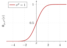
The central limit theorem says that the distribution of an average of many independent, identically distributed random variables tends toward the famous bell-shaped normal distribution with a probability density function of:

where μ is the expected value of the random variables, σ equals their distribution's standard deviation divided by n1/2, and n is the number of random variables. The standard deviation therefore is simply a scaling variable that adjusts how broad the curve will be, though it also appears in the normalizing constant.
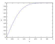
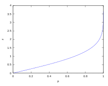
If a data distribution is approximately normal, then the proportion of data values within z standard deviations of the mean is defined by:
- Proportion =

where is the error function. The proportion that is less than or equal to a number, x, is given by the cumulative distribution function:

- Proportion ≤ .[11]
![x={\frac {1}{2}}\left[1+\operatorname {erf} \left({\frac {x-\mu }{\sigma {\sqrt {2}}}}\right)\right]={\frac {1}{2}}\left[1+\operatorname {erf} \left({\frac {z}{\sqrt {2}}}\right)\right]](../I/m/92a80077c1c5100697c8e560d88d846ebffd3040.svg)
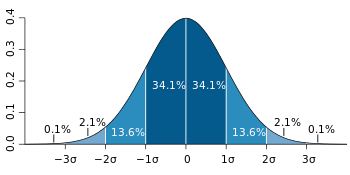
If a data distribution is approximately normal then about 68 percent of the data values are within one standard deviation of the mean (mathematically, μ ± σ, where μ is the arithmetic mean), about 95 percent are within two standard deviations (μ ± 2σ), and about 99.7 percent lie within three standard deviations (μ ± 3σ). This is known as the 68-95-99.7 rule, or the empirical rule.
For various values of z, the percentage of values expected to lie in and outside the symmetric interval, CI = (−zσ, zσ), are as follows:
| Confidence interval |
Proportion within | Proportion without | |
|---|---|---|---|
| Percentage | Percentage | Fraction | |
| 0.674490σ | 50% | 50% | 1 / 2 |
| 0.994458σ | 68% | 32% | 1 / 3.125 |
| 1σ | 68.2689492% | 31.7310508% | 1 / 3.1514872 |
| 1.281552σ | 80% | 20% | 1 / 5 |
| 1.644854σ | 90% | 10% | 1 / 10 |
| 1.959964σ | 95% | 5% | 1 / 20 |
| 2σ | 95.4499736% | 4.5500264% | 1 / 21.977895 |
| 2.575829σ | 99% | 1% | 1 / 100 |
| 3σ | 99.7300204% | 0.2699796% | 1 / 370.398 |
| 3.290527σ | 99.9% | 0.1% | 1 / 1000 |
| 3.890592σ | 99.99% | 0.01% | 1 / 10000 |
| 4σ | 99.993666% | 0.006334% | 1 / 15787 |
| 4.417173σ | 99.999% | 0.001% | 1 / 100000 |
| 4.5σ | 99.9993204653751% | 0.0006795346249% | 3.4 / 1000000 (on each side of mean) |
| 4.891638σ | 99.9999% | 0.0001% | 1 / 1000000 |
| 5σ | 99.9999426697% | 0.0000573303% | 1 / 1744278 |
| 5.326724σ | 99.99999% | 0.00001% | 1 / 10000000 |
| 5.730729σ | 99.999999% | 0.000001% | 1 / 100000000 |
| 6σ | 99.9999998027% | 0.0000001973% | 1 / 506797346 |
| 6.109410σ | 99.9999999% | 0.0000001% | 1 / 1000000000 |
| 6.466951σ | 99.99999999% | 0.00000001% | 1 / 10000000000 |
| 6.806502σ | 99.999999999% | 0.000000001% | 1 / 100000000000 |
| 7σ | 99.9999999997440% | 0.000000000256% | 1 / 390682215445 |
Relationship between standard deviation and mean
The mean and the standard deviation of a set of data are descriptive statistics usually reported together. In a certain sense, the standard deviation is a "natural" measure of statistical dispersion if the center of the data is measured about the mean. This is because the standard deviation from the mean is smaller than from any other point. The precise statement is the following: suppose x1, ..., xn are real numbers and define the function:

Using calculus or by completing the square, it is possible to show that σ(r) has a unique minimum at the mean:

Variability can also be measured by the coefficient of variation, which is the ratio of the standard deviation to the mean. It is a dimensionless number.
Standard deviation of the mean
Often, we want some information about the precision of the mean we obtained. We can obtain this by determining the standard deviation of the sampled mean. Assuming statistical independence of the values in the sample, the standard deviation of the mean is related to the standard deviation of the distribution by:

where N is the number of observations in the sample used to estimate the mean. This can easily be proven with (see basic properties of the variance):

hence

Resulting in:

It should be emphasized that in order to estimate standard deviation of the mean it is necessary to know standard deviation of the entire population beforehand. However, in most applications this parameter is unknown. For example, if series of 10 measurements of previously unknown quantity is performed in laboratory, it is possible to calculate resulting sample mean and sample standard deviation, but it is impossible to calculate standard deviation of the mean.


Rapid calculation methods
The following two formulas can represent a running (repeatedly updated) standard deviation. A set of two power sums s1 and s2 are computed over a set of N values of x, denoted as x1, ..., xN:

Given the results of these running summations, the values N, s1, s2 can be used at any time to compute the current value of the running standard deviation:

Where N, as mentioned above, is the size of the set of values (or can also be regarded as s0).
Similarly for sample standard deviation,

In a computer implementation, as the three sj sums become large, we need to consider round-off error, arithmetic overflow, and arithmetic underflow. The method below calculates the running sums method with reduced rounding errors.[12] This is a "one pass" algorithm for calculating variance of n samples without the need to store prior data during the calculation. Applying this method to a time series will result in successive values of standard deviation corresponding to n data points as n grows larger with each new sample, rather than a constant-width sliding window calculation.
For k = 1, ..., n:

where A is the mean value.

Note: since or


Sample variance:

Population variance:

Weighted calculation
When the values xi are weighted with unequal weights wi, the power sums s0, s1, s2 are each computed as:

And the standard deviation equations remain unchanged. Note that s0 is now the sum of the weights and not the number of samples N.
The incremental method with reduced rounding errors can also be applied, with some additional complexity.
A running sum of weights must be computed for each k from 1 to n:

and places where 1/n is used above must be replaced by wi/Wn:

In the final division,

and

or

where n is the total number of elements, and n' is the number of elements with non-zero weights. The above formulas become equal to the simpler formulas given above if weights are taken as equal to one.
History
The term standard deviation was first used[13] in writing by Karl Pearson[14] in 1894, following his use of it in lectures. This was as a replacement for earlier alternative names for the same idea: for example, Gauss used mean error.[15]
See also
- 68–95–99.7 rule
- Accuracy and precision
- Chebyshev's inequality An inequality on location and scale parameters
- Cumulant
- Deviation (statistics)
- Distance correlation Distance standard deviation
- Error bar
- Geometric standard deviation
- Mahalanobis distance generalizing number of standard deviations to the mean
- Mean absolute error
- Pooled standard deviation
- Percentile
- Raw score
- Relative standard deviation
- Robust standard deviation
- Root mean square
- Sample size
- Samuelson's inequality
- Six Sigma
- Standard error
- Standard score
- Volatility (finance)
- Yamartino method for calculating standard deviation of wind direction
References
- ↑ Bland, J.M.; Altman, D.G. (1996). "Statistics notes: measurement error". BMJ. 312 (7047): 1654. doi:10.1136/bmj.312.7047.1654. PMC 2351401
 . PMID 8664723.
 - ↑ Gauss, Carl Friedrich (1816). "Bestimmung der Genauigkeit der Beobachtungen". Zeitschrift für Astronomie und verwandte Wissenschaften. 1: 187–197.
- ↑ Walker, Helen (1931). Studies in the History of the Statistical Method. Baltimore, MD: Williams & Wilkins Co. pp. 24–25.
- ↑ Gorard, Stephen. Revisiting a 90-year-old debate: the advantages of the mean deviation. Department of Educational Studies, University of York
- ↑ Weisstein, Eric W. "Bessel's Correction". MathWorld.
- ↑ "CERN | Accelerating science". Public.web.cern.ch. Retrieved 2013-08-10.
- ↑ "CERN experiments observe particle consistent with long-sought Higgs boson | CERN press office". Press.web.cern.ch. 2012-07-04. Retrieved 2015-05-30.
- ↑ LIGO Scientific Collaboration, Virgo Collaboration (2016), "Observation of Gravitational Waves from a Binary Black Hole Merger", Physical Review Letters, 116 (6): 061102, arXiv:1602.03837, doi:10.1103/PhysRevLett.116.061102
- ↑ "What is Standard Deviation". Pristine. Retrieved 2011-10-29.
- ↑ Ghahramani, Saeed (2000). Fundamentals of Probability (2nd Edition). Prentice Hall: New Jersey. p. 438.
- ↑ Eric W. Weisstein. "Distribution Function". MathWorld—A Wolfram Web Resource. Retrieved 2014-09-30.
- ↑ Welford, BP (August 1962). "Note on a Method for Calculating Corrected Sums of Squares and Products" (PDF). Technometrics. 4 (3): 419–420. doi:10.1080/00401706.1962.10490022.
- ↑ Dodge, Yadolah (2003). The Oxford Dictionary of Statistical Terms. Oxford University Press. ISBN 0-19-920613-9.
- ↑ Pearson, Karl (1894). "On the dissection of asymmetrical frequency curves". Philosophical Transactions of the Royal Society A. 185: 71–110. doi:10.1098/rsta.1894.0003.
- ↑ Miller, Jeff. "Earliest Known Uses of Some of the Words of Mathematics".
External links
- Hazewinkel, Michiel, ed. (2001), "Quadratic deviation", Encyclopedia of Mathematics, Springer, ISBN 978-1-55608-010-4
- A simple way to understand Standard Deviation
- Standard Deviation – an explanation without maths
- The concept of Standard Deviation is shown in this 8-foot-tall (2.4 m) Probability Machine (named Sir Francis) comparing stock market returns to the randomness of the beans dropping through the quincunx pattern. on YouTube from Index Funds Advisors IFA.com
| |||||||||||||||||||||||||||||||||||||||||||||
| |||||||||||||||||||||||||||||||||||||||||||||
| |||||||||||||||||||||||||||||||||||||||||||||
| |||||||||||||||||||||||||||||||||||||||||||||
| |||||||||||||||||||||||||||||||||||||||||||||
| |||||||||||||||||||||||||||||||||||||||||||||
| |||||||||||||||||||||||||||||||||||||||||||||